
In this phase, the possible alternative options – i.e. the Responses in terms of the DPSIR framework – are defined in terms of their performances. The criteria for evaluating performance are determined based on the available indicators. For each possible option scenario, the user must assign a corresponding value to each criterion. Those indicator values relevant for decision making, either coming from model outcomes or from other sources, are organised in the form of a matrix – the Analysis Matrix (AM) – containing the indicator values of the alternative options (in the columns) for each decision criterion (in the rows). At this stage, the indicator values are measured in different units and scales. In the next phase, indicator values are made comparable by normalisation and/or by the application of value functions and used to fill the Evaluation Matrix (EM).
The Analysis Matrix (AM)
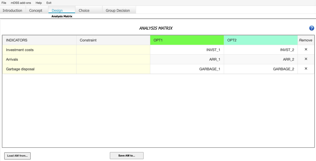
The Analysis Matrix (AM) is a tabular representation of indicator values representing the outcomes of previous assessments of the expected performances of the alternative options (i.e. the set of Responses identified in the DPSIR Frame) measured in natural units (such as kg/yr, m3, ppm etc.). An example of an Analysis Matrix (AM) related to the case study of Auronzo di Cadore, within the scalar context, is presented in Figure 17.
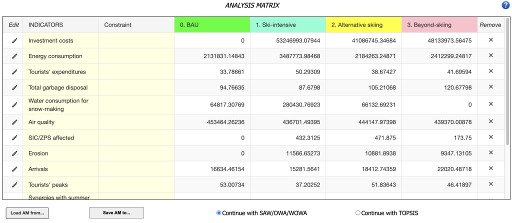
On the right side of the AM Window, the responses are listed. Once filled with data, the numbers inside the matrix represent the indicator values of the alternative options for each decision criterion and are measured in different units and scales. In the SOS and MOS cases, the visualization of the AM differs slightly due to the multidimensional nature of the .dbf structure. Specifically, the values are not directly visible because the elements of the AM are vectors that define the indicator values for a given alternative across all analyzed spatial objects.
The “Constraint” column allows the user to define both a maximum and a minimum value for the indicators considered. If a value exceeds these limits—whether above the maximum or below the minimum—mDSS truncates it to fit within the specified boundaries.
From Concept to Design
Depending on the analysis methods selected (scalar, MOS, or SOS), the steps to generate the Analysis Matrix (AM) in the mDSS may differ. The following sub-sections offer a detailed, method-specific explanation of these steps, continuing from where the discussion was paused in the previous chapter.
1. Multi-Criteria Analysis (MCA)
After uploading the Catalogue of DPSIR Indicators and the Catalogue of Response Measures, the user must select which indicators to include in the quantitative analysis of the measures. Additionally, the user is required to assign values to these indicators for each alternative scenario.
To select the indicators to include in the Analysis Matrix (AM), the user must navigate to the DPSIR window (shown in Figure 6, in the Concept section of the Tab Bar). In this window, the user should right-click on the name of each indicator and select “Send ‘X’ to AM Matrix.” Once the indicator is sent to the AM Matrix, the colour of its name in the DPSIR window changes from black to red. This visual change helps easily identify which indicators contribute to the results of the quantitative analysis.
Once the desired indicators are sent to the AM from the Concept Phase window, the user must select “Design” in the Tab Bar to visualize the matrix. The user will then see a table similar to the one shown in Figure 17, although the cells for the values will initially be empty.
In mDSS, the cells of the AM in the scalar can be populated in various ways:
- by loading a pre-existing matrix from a .xlsx file using the “Load AM from…” button;
- by manually entering values, which can be done by clicking the “pencil” icon in the “Edit” column to modify or insert values;
- by right-clicking on the name of the indicator in the DPSIR window and selecting “Set values from…”.
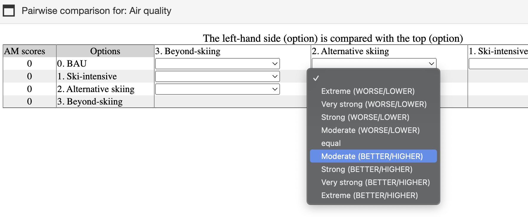
With option (3), the user can assign values to individual indicators, or to a subgroup of them, for both “Pairwise Comparison of Options” and “Hierarchical Comparison of Options.” This process effectively converts qualitative assessments into quantitative data. For example, by right-clicking on the “Air Quality” indicator and selecting “Pairwise Comparison of Options,” mDSS opens a window similar to the one shown in Figure 18. To obtain a quantitative evaluation of the indicator’s values, the user should compare the different options based on the chosen indicator (e.g., Air Quality). For instance, if the user selects “moderate (BETTER/HIGHER)” from the drop-down menu in Figure 18, it indicates that they believe the air quality in Option 0 is slightly better than in Option 2. Note that this method requires a certain threshold of consistency in the matrix, which ensures that the comparisons between options are logically coherent. If the Consistency Index exceeds 0.1, mDSS will block the user from proceeding until the matrix is corrected. For further explanation concerning consistency, please refer to the Methods Handbook.
The mDSS also provides a “Hierarchical Comparison of Options” feature, which adds an extra level of hierarchy between options during the comparison process. To begin, after selecting “Hierarchical Comparison of Options,” the user should click the “Start Select” button in the “Hierarchical Weighting” window. Once the options to be aggregated are chosen, they will turn pink. After completing the aggregation, the user should click the “End Select” button, give a name to the new macro-option, and a Pairwise Comparison of Options window, similar to the one shown in Figure 18, will appear. Upon finishing the process, the user should click “Ok” to assign values to the selected indicator, converting qualitative statements into quantitative data. Finally, the user can click on “File” and choose one of the following options: “Save the Structure,” “Save the Image,” or “Load a Structure.”
Once the Analysis Matrix is created, the user can remove a row (i.e., an indicator) by clicking the “x” icon in the last column. Once the structure of the AM has been defined, the cells of the matrix should be filled with indicator values using one of the three methods described above.

Once the AM Matrix is ready, the user can choose which aggregation algorithm to use for continuing the analysis: SAW/OWA/WOWA, or TOPSIS. The default algorithm is SAW. The next steps involve creating the Evaluation Matrix (EM) based on the Analysis Matrix (AM) and proceeding with the option selection. To pass to the Choice phase, the user must click the “Choice” button in the Tab bar. A detailed explanation of the steps required for this phase is provided in the next chapter.
Before proceeding to the next stage of the process, it is advisable to save the final version of the Analysis Function (AM) by clicking on the button “Save AM to…”. This ensures no information is lost and creates a .xlsx file that can be easily uploaded in future sessions.
2. Multi-Criteria Spatial Scenario (MSS)
As in the scalar context, after uploading the Catalogue of DPSIR Indicators and the Catalogue of Response Measures, the user must select which indicators to include in the quantitative analysis of the measures. Additionally, the user is required to assign values to these indicators for each alternative scenario.
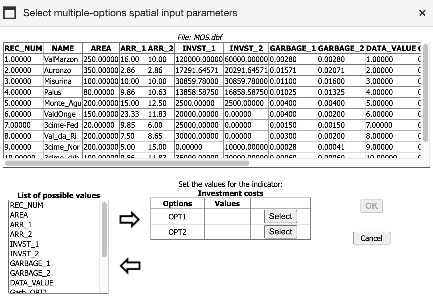
The primary difference from the scalar case is that the indicator values for the quantitative analysis have already been uploaded into mDSS toward the .dbf file. To match the indicator uploaded in the Catalogue of DPSIR Indicators with the corresponding columns in the .dbf file, the user must right-click on one of the indicator names in the DPSIR window and select “Set values”. An example of this procedure referring to the case study of Auronzo di Cadore is shown in Figure 20. After clicking on it, mDSS will propose a window similar to the one reported in Figure 21.
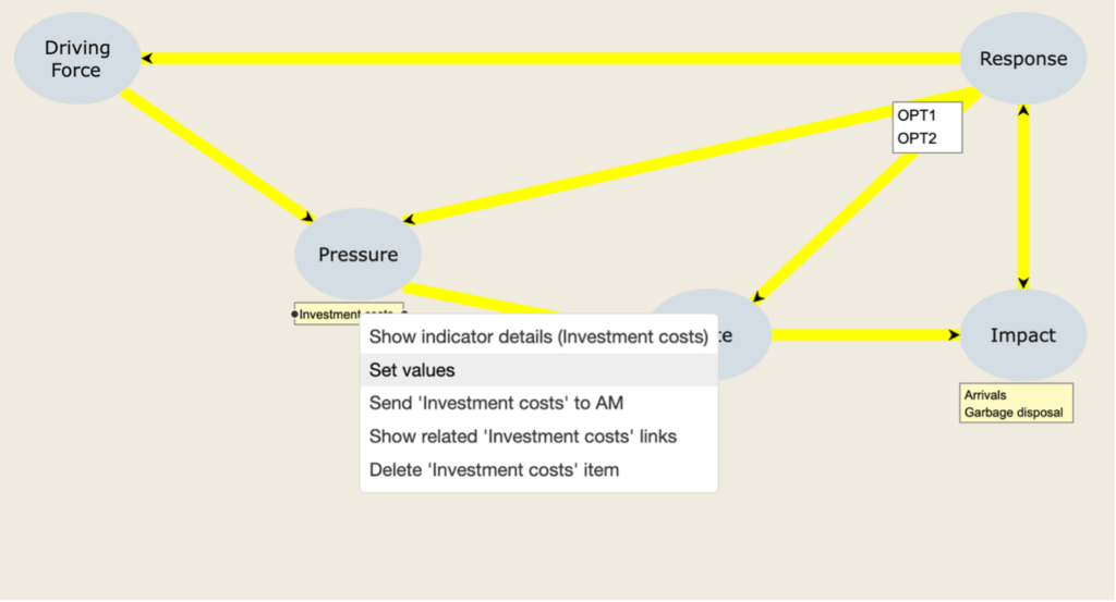
In this example, the user selects the indicator “Investment costs”. To proceed, they must specify which column in the .dbf file corresponds to the indicator’s value for the first option and which column corresponds to the second option. Note that “OPT1” and “OPT2” refer to the names of the options uploaded by the user in the Catalogue of Response Measures.
To assign the indicator values for OPT1, the user should follow these steps:
- Click the “Select” button on the right-hand side.
- In the left-hand “List of Possible Values”, locate and select the name of the .dbf column that corresponds to Investment Costs for OPT1. In this case, it is “INVST_1”.
- Click the right-directed arrow to assign the selected column. The column name will then appear under the “Values” field.
Then, repeat the process for OPT2.
To remove a .dbf column from the “Values” field:
- Click “Select.”
- Click the left-directed arrow.
By clicking “OK”, mDSS will return the user to the standard DPSIR framework. This process should be repeated for each indicator available in the .dbf columns, or at minimum, for those that will be selected for the quantitative analysis.
Notably, assigning values to the indicators does not automatically send the indicator to the Analysis Matrix (AM). Once the “Set values” process is completed for an indicator, the user can include it in the quantitative analysis by right-clicking on the indicator’s name in the DPSIR window and selecting “Send ‘X’ to AM”.
After completing this process for all relevant indicators, the user can proceed to the Choice phase by clicking the “Choice” button in the Tab bar. A detailed explanation of the steps for this phase can be found in the next chapter.
3. Multi-Criteria Suitability Analysis (MSA)
In the MSA case, the Analysis Matrix will automatically be prepared once the DPSIR framework is completed, incorporating the indicators selected during the Concept phase. To access the Analysis Matrix, the user should click the “Design” button in the Tab Bar. This action will open a window similar to the one shown in Figure 23.
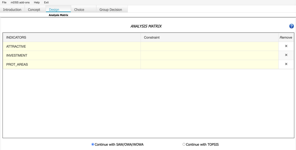
If the user has also uploaded .shp and .shx data, clicking on the indicator name in the Analysis Matrix (AM) will display a geographical representation of the selected indicator’s values. For instance, by selecting “INVESTMENT” in Figure 23, mDSS will present a window similar to the one shown in Figure 24.

As with other methods, before proceeding to the Choice phase, the user must specify their preference for either the SAW/OWA/WOWA method or the TOPSIS method. Once a selection has been made, the user should click the “Choice” button in the Tab Bar to initiate the Choice phase.