The comparison of the alternative options is the final phase of the decision-making process adopted by mDSS. Using multi-criteria analysis evaluation techniques, all options are judged, against their performances according to the set of indicators identified in the AM. The main aim of MCA methods is to reduce the “multidimensionality” of decision problems – the multivariate option performances – into a single measure enabling an effective ranking. The heart of any MCA decision rule is therefore an aggregation procedure.
Decision rules combine partial preferences, derived from the performance of individual criteria, into a global preference score. This aggregated score facilitates the ranking of the alternative options under consideration. There is no single method universally suitable for any kind of decision problem. mDSS provides four decision rules:
- Simple Additive Weighting (SAW);
- Ordered Weighting Average (OWA),
- Weighted Ordered Weighting Average (WOWA),
- The Technique for Order Preference by Similarity to Ideal Solution (TOPSIS).
Normalising the values: from AM to EM
The first step of the Choice phase involves normalizing the values in the Analysis Matrix (AM). This is essential because the AM contains values expressed in different units of measurement. Defining the Value Function is necessary for the methods SAW, OWA, and WOWA. For the TOPSIS method, normalization is handled automatically as part of the method’s construction.
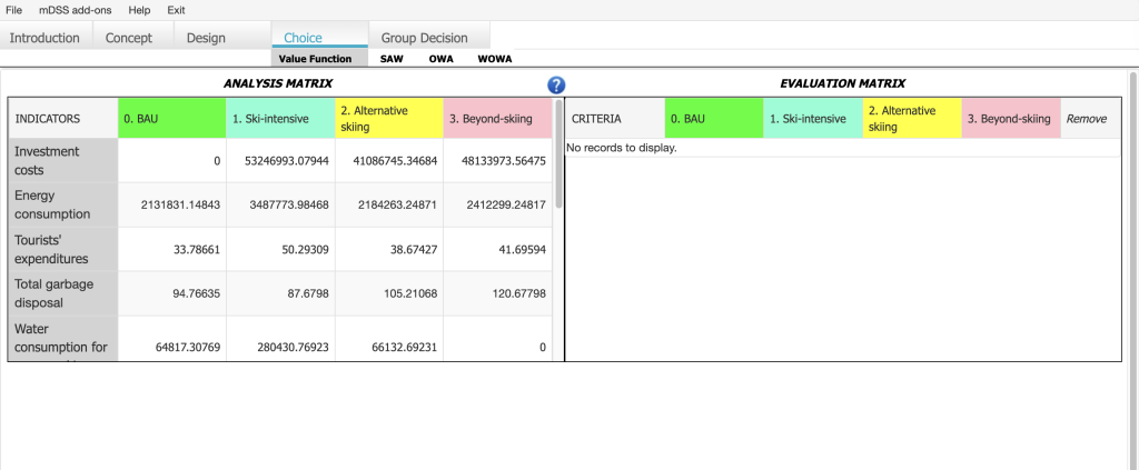
The value function window can be opened by clicking on the Choice Tab of the Tab Bar, and this is true for all three analysis contexts (scalar, MOS and SOS). During the work session, the user can process the data contained in the Analysis Matrix (AM) to produce the Evaluation Matrix (EM). After clicking on “Choice”, if the user selects SAW/OWA/WOWA in the previous step, a Value Function Window will appear, similar to the one shown in Figure 25. While Figure 25 illustrates the scalar context, the subsequent normalisation process can be generalised to the other two contexts as well.
The Value Function Window contains both the analysis and the evaluation matrices. Initially, the evaluation matrix sub-window, (on the right of the program window), is empty. The user must individually select every row of the AM by clicking on the name of the indicator, check one of the standardise options (Value Function, Benefit type, Cost type at the bottom-right of the window) in order to define the standardisation function, and, once the function is defined, press the “Send to EM” button to build the EM. At the end of this process, the EM contains the normalised values of the analysis matrix – the values in each row of the analysis matrix transformed to a common [0, 1] range.
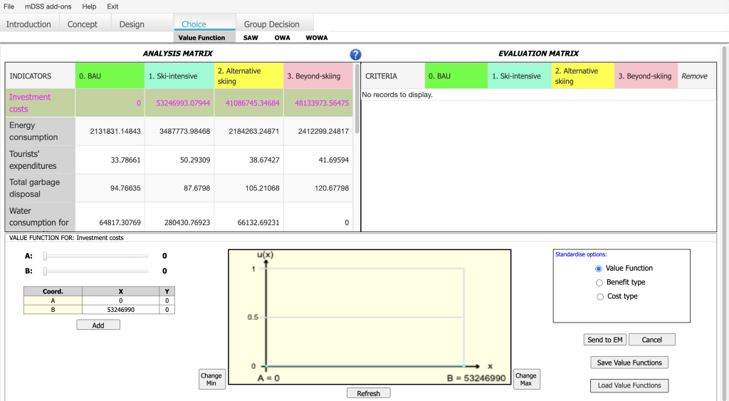
As previously mentioned, to begin the normalization process for a specific indicator, the user should click on the indicator’s name within the Analysis Matrix. For instance, to normalize the indicator “Investment costs,” the user needs to click on its name located in the leftmost grey column labelled Indicators. Once selected, the value function sub-window will appear at the bottom of the screen, as shown in Figure 26.
The transformation of multidimensional indicators stored in the Analysis Matrix into evaluation indices for the Evaluation Matrix is a crucial step. In this process, the decision maker assesses the performance of the alternative options (i.e., the Responses within the DPSIR framework) based on the data measured or estimated in the Analysis Matrix. This assessment reflects preferences specific to the decisional case under examination.
The decision maker’s judgment is expressed through a value function, which converts the Analysis Matrix data (expressed in natural units such as m³, t, etc.) into normalized values ranging from 0 to 1. This transformation ensures that the evaluation criteria are on a comparable scale.
Three alternative forms of the linear value function (“Standardise options” in Figure 26) are available in mDSS:
- By selecting the “Value Function” option, the user can create a variety of piecewise-linear value functions, such as a trapezoidal function. The parameters of the value function (A and B) define the first and last points of the model, which correspond to the minimum and maximum observed values of the selected indicators. To modify the value curve, the user can click on the pale blue line in the graphic to add new points, which will define the shape of the curve. These points will be displayed in the table on the left. Editing is completed by double-clicking and selecting the “Stop” button. Alternatively, the user can edit the curve by clicking the “Add Button” and manually entering coordinates. If the user wishes to restart the process, they can simply click the “Refresh” button. The red line in the graph represents the previously created Value Function for that indicator;
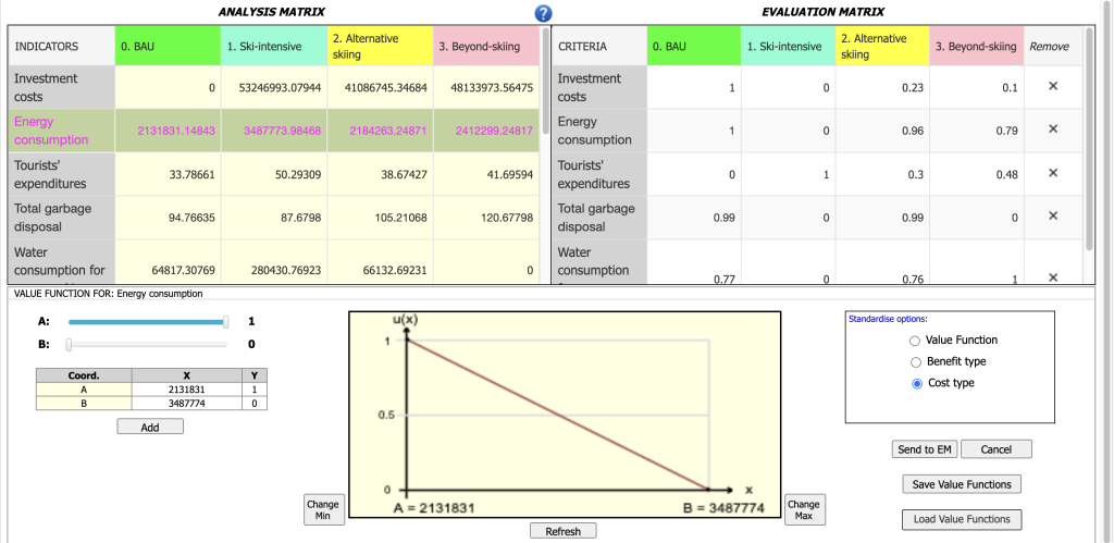
- By selecting the “Benefit Type” option, the user can transform the AM data (expressed in natural units) through min-max normalization. This process applies a linear transformation to the data in the selected AM row, assigning a value of 0 to the minimum value and 1 to the maximum value of the row;
- By selecting the “Cost Type” option, min-max normalization is applied with a reversed scale, where a value of 0 is assigned to the maximum value of the row, and 1 is assigned to the minimum value.
On the left side of the screen, the user can find two rulers, A and B, that allow the user to move the coordinates of the two points on the y-axis. Using the buttons on the bottom right side of the window, the user can save and load value functions. The value functions are saved in a .xlsx file.
By default, the value functions are set between the minimum and maximum values of the row in the AM. If the user needs to adjust this range—such as to focus on an optimal interval or expand it to encompass a broader set of values—the value functions can be modified in two ways:
- Using the Change Min and Change Max buttons: These buttons, located on the left and right sides of the value function plot, allow the user to adjust the extremes of the function directly.
- Manually: Save the value functions as an .xlsx file, modify the extreme values in Excel, and then re-load the modified file into mDSS.
Note: The user is advised to save the value functions. When one or more criterion values are modified in the analysis matrix, the modified criteria are automatically removed from the EM. As a result, the value functions that rely on these modified criteria will be cancelled. The user will only be able to reload the Analysis Matrix (AM) if it has been saved previously. If the AM has not been saved, the user will need to re-enter the values.
In the sub-window shown in Figure 26–27, the red line represents the last Value Function saved in the .mD5 file for the indicator, while the light blue line represents the current one. The red line is purely graphical and does not influence the process.
An example of a completed Evaluation Matrix (EM) is shown in Figure 27. Once the process is finished, the user should click on the SAW button located at the top of the screen, just below the Tab Bar, where they can input the criteria importance weights.
In the context of MSS and MSA, if the user has uploaded .shp and .shx files, clicking on an indicator name in the Evaluation Matrix will display a spatial map showing the normalized values of the selected indicator, similar to what is shown in Figure 24 for the Analysis Matrix.
Assigning importance weights
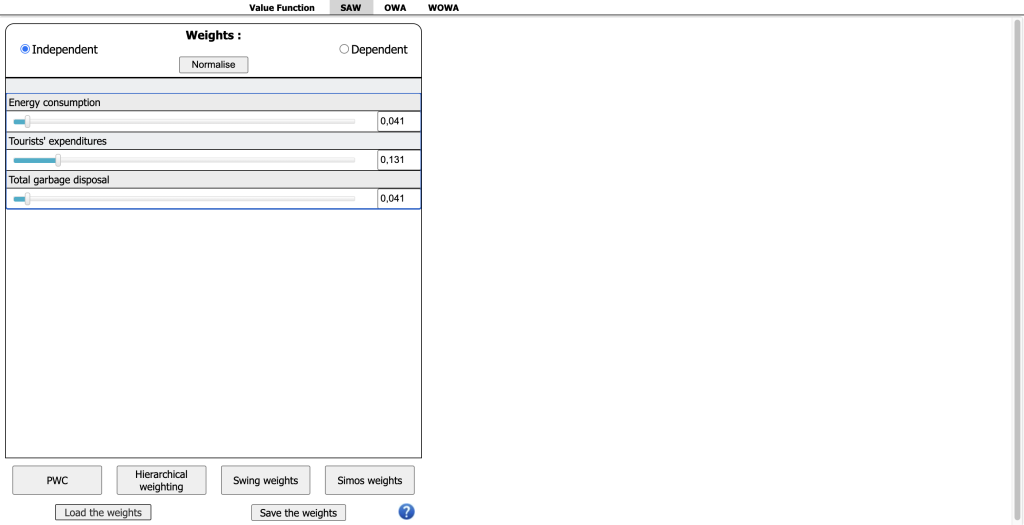
Once the Evaluation Matrix is complete, the user can proceed to the weight assignment session in the SAW section. To do this, click the SAW button located at the top of the screen, just below the Tab Bar. Upon clicking, a window similar to the one shown in Figure 28 will appear. After the importance weights have been entered and normalized, mDSS will display the option rankings based on the SAW algorithm on the right side of the screen.
In this step, the decision maker indicates the relative importance of each criterion stored in the EM for the decision at hand. The weighting process generates a vector of weights, which can be saved using the “Save Weights” button in a separate file (.wgt file) and reloaded in future sessions with the “Load Weights” button. These functions are useful for refining the model or comparing the preferences of different stakeholders, particularly in group decision-making. After assigning weights, the decision outcomes can be aggregated according to the decision maker’s preferences.
The methodology path varies depending on the decision rule (SAW, OWA, WOWA, or TOPSIS) selected earlier, as explained in the following sections. Generally, in mDSS, the criterion weights can be defined in multiple ways:
- Independent
- Dependent
- Pairwise Comparison Weighting
- Hierarchical Weighting
- Swing Weights
- Simos Weight
1. Independent
The weights can be defined independently (by activating the “Independent” option in the weight quadrant) by adjusting the sliders, manually entering values, or using the up-down arrows. They must then be normalised by pressing the “Normalise” button, ensuring their sum equals one. The resulting weight vector can be saved in a .wgt file for further use.
2. Dependent
The weights can be defined in a dependent way (by activating the “Dependent” option), where changes to one weight are interactively linked to changes in all other weights, proportional to their values.
3. Pairwise Comparison Weighting
The weights can also be defined using the Pairwise Comparison Weighting approach (via the “PWC” button). In this approach, the user is asked to compare each pair of criteria individually. For each pair, the user indicates how important the criterion in the row is relative to the criterion in the column. Once the comparison matrix is completed, the associated criteria weights are calculated and displayed in the first column. Since pairwise comparisons may generate inconsistencies, the consistency index (see the Methods Handbook), located at the bottom of the display, serves as a guide. If the index value is below 0.1, the matrix is considered sufficiently consistent. Otherwise, the user should revise the comparisons. If the matrix is consistent, clicking the “OK” button copies the calculated weights into the weight quadrant (sliders), where they can still be interactively adjusted and their effect visually examined. The weights can then be saved in a .wgt file for further use.
4. Hierarchical Weighting
They may be defined by using the Hierarchical Weighting approach, in which weights are assigned by comparing subsets of criteria, which are then grouped into macro-criteria at various possible levels of hierarchy. The pairwise comparison approach is also used in this case but with the advantage of being applied to smaller subsets of criteria. This facilitates comparisons because criteria within a subset are usually more homogeneous and thus more easily comparable (e.g. various forms of pollution). At higher hierarchical levels macro-criteria are compared to each other in new matrices. The higher the hierarchical level, the lower is usually the technical content of the comparison and the higher the political meaning (e.g. deciding the relative weight of pollution as compared to unemployment).
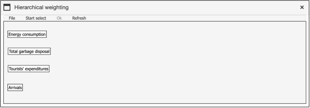
To initiate the Hierarchical Weighting process, the user clicks the “Start Select” button located in the “Hierarchical Weighting” window (Figure 29). Once the user has selected the criteria to be aggregated in a macro-criterion, the selected criteria will turn pink. When the aggregation is thought to be finished, the user is requested to click on the “End Select” button to type the name of the new macro-criterion and to assign the weights to the chosen criteria. At every hierarchical level, the criteria previously selected are highlighted in yellow and no longer available for hierarchical aggregation. By right-clicking on any of the created aggregated nodes, the user can perform the following actions: delete the node, rename it, or modify the pairwise comparison matrix.
An example of a simple, completed hierarchical structure is shown in Figure 30. Once the structure is finalised, the user can click on “File” and choose one of the following options: “Save the structure“, “Upload a previously developed structure“, or “Save the structure representation as an image“.
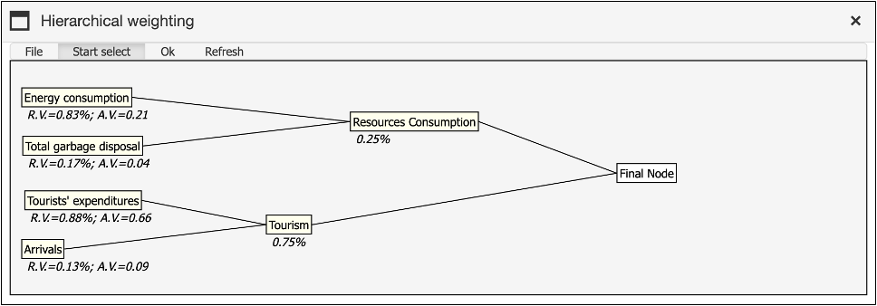
At the conclusion of the hierarchical process, clicking the “OK” button copies the calculated weights into the weight quadrant (sliders). These weights can still be adjusted interactively, allowing users to visualise the effects of changes before saving them as a .wgt file for further analysis.
5. Swing Weights
They may be defined using the Swing Weights procedure. The algorithm relies on the “swing,” which represents the change in performance from the worst to the best outcome of a given criterion. Swings are calculated separately for each criterion.
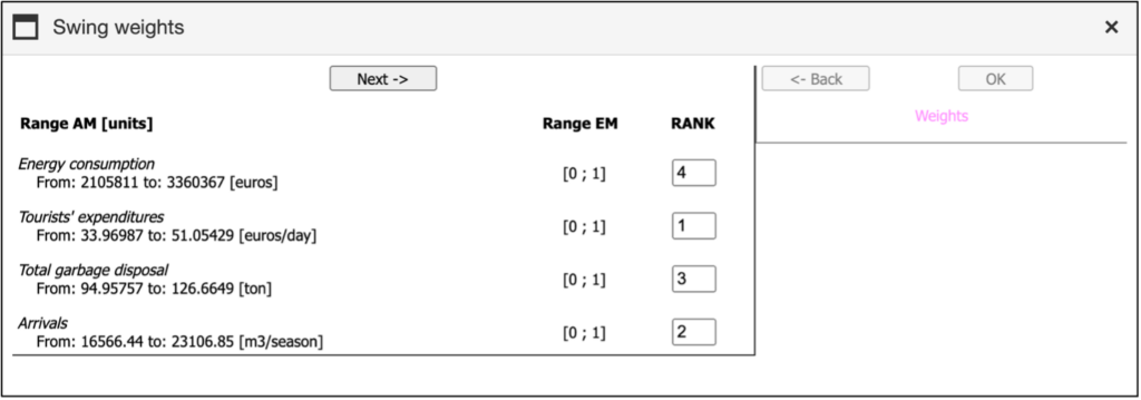
The swing weights window is divided into two sections: The first section displays the decision criteria, along with their ranges before and after normalization (i.e., values from both the Analysis Matrix and the Evaluation Matrix), as well as the rank position of each criterion. Users must assign rank positions to the criteria in this section to proceed to the second section, where the weights are elicited. It is important to note that each rank position can only be assigned to one criterion.
When the user clicks on the “Swing weights” button, the first of two panels will open, as shown in Figure 31. In this panel, the user must first define the rank position for all criteria. To do this, they can either click into the text field and edit the number directly or use the arrow buttons beneath the text field to adjust the rank. The most important criterion is that for which the change from the worst to the best outcome represents the highest increase in the total performance. The user should assign rank 1 to this criterion, rank 2 to the second most important criterion and so on until the rank of the least important criterion (n) is defined. Once all ranks are assigned, the “Next” button will become active, allowing the user to proceed.
After clicking the “Next” button, the second part of the window opens. This section contains several sliders, each corresponding to a different criterion. The sliders allow users to assign relative importance to each criterion by adjusting the slider position. The range for each slider is calculated by the program based on the criterion ranking defined by the user in the left panel. By default, the program sets the weights to the middle of the allowed interval. An example is reported in Figure 32.
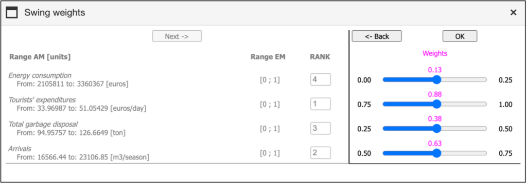
When the user is satisfied with the adjustments, they can click the “OK” button at the top of the panel to return to the SAW window with the non-normalized weights. If the user wishes to return from the right panel to the left panel, they can use the “Back” button.
Example: Suppose you have up to 100 points to assign to each criterion, based on the performance change from the worst to the best outcome. If the swing (change) for the most important criterion is assigned 100 points, how many points would you assign to the second most important criterion? To make your selection, move the slider to the appropriate position. Repeat this process for all other criteria. Once you have finished, click “OK” to finalize your choices. The criteria weights will be calculated based on your selections, and the results will be displayed in the standard window. For a more detailed explanation, see the Methods Handbook.
6. SIMOS weight
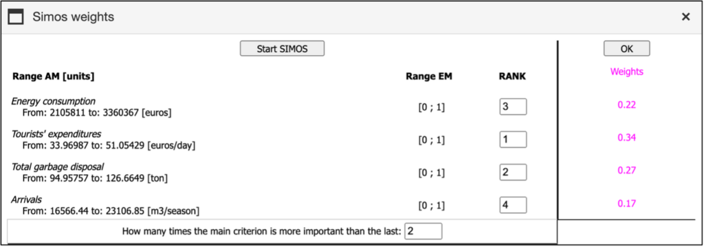
The weights can be defined using the SIMOS weight procedure. The user must assign an importance ranking to each criterion, with two or more criteria able to share the same rank. Finally, the user needs to specify in the last cell how many times the weight of the most important criterion (rank = 1) should be greater than that of the least important criterion. mDSS will then calculate the remaining weights based on these two boundaries (Figure 33). At the end of the process, clicking the “OK” button transfers the calculated weights into the weight quadrant (sliders). These weights can still be interactively adjusted, allowing users to visualize the impact of changes before saving them as a .wgt file for further analysis.
Decision Rules
In order to establish a ranking of the alternatives, the partial scores describing the performance of each alternative in respect to each single criterion should be aggregated. Such aggregation can be done by following different decision rules. In mDSS are available the following types of decision rules:
- Simple Additive Weighting (SAW);
- Ordered Weighting Average (OWA),
- Weighted Ordered Weighting Average (WOWA),
- The Technique for Order Preference by Similarity to Ideal Solution (TOPSIS).
The user can select the Decision Rule in the Analysis Matrix (AM) window (SAW/OWA/WOWA or TOPSIS). In the first case, even if she/he intends to use OWA or WOWA, she/he must first go through the SAW window to set the importance weights as described earlier.
1. Simple additive weighting (SAW)
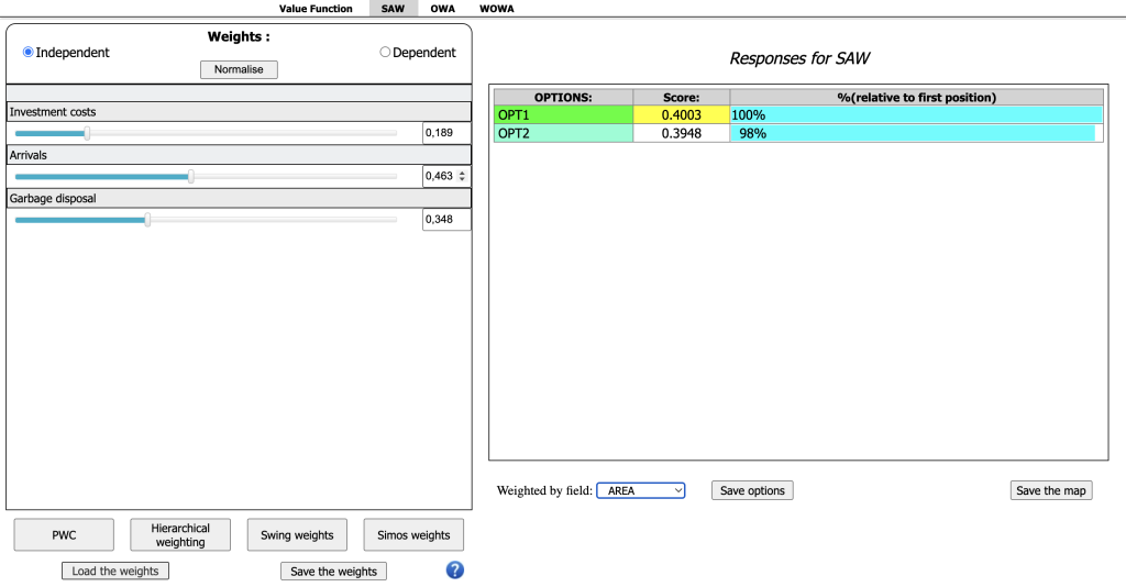
SAW is a simple sum of the criterion values of every option, weighted by the vector of weights. The results are represented as scores, and the option with the highest score is considered the most preferred
Once the vector of criteria weights is defined, and after clicking on “Normalize,” the Response for SAW will appear on the right side of the SAW window. The score of the best option is coloured in yellow. The others are ranked according to their absolute score and their % relative to the first position. Figure 34 reports an example of Responses for SAW.

The ranking of options can be saved in a separate file (.opt file) by clicking on the “Save options” button. In this way it will be possible, for instance, to compare the rankings obtained from different analyses, e.g. different actors or different decision rules.
Once the ranking is displayed, the user can access useful graphical visualizations of the results and perform a sensitivity analysis. For more information, please refer to the dedicated section.
Notably, in the MSS context, the interface for “Responses for SAW” (as well as for OWA, WOWA, and TOPSIS) behaves slightly differently. Specifically, after the user clicks on “Normalise,” a ranking does not immediately appear, as shown in Figure 34. Instead, two additional buttons appear, as illustrated in Figure 35.

At this point, the user can click on “Save the map” to download a .zip file containing a .shp file, a .shx file, and a .dbf file. These files contain the ranking results for each spatial object. In the context of the Auronzo di Cadore case study, importing these files into GIS software allows the user to visualise the disaggregated ranking results for each single zone.
To generate a single, unified ranking that identifies the best solution across all areas, the user can weight the SAW “local” scores of each alternative for every spatial object using a variable stored in the .dbf file, such as the area of each zone. By aggregating these weighted scores, a unique global ranking of the alternatives is produced. Figure 36 illustrates an example of this process as applied to the case study. To select the appropriate weighting variable, the user needs to click on the “Weighted by field” button and choose from the available list.
Once the global ranking is calculated, the user can save it as a .opt file by clicking the “Save Options” button that appears.
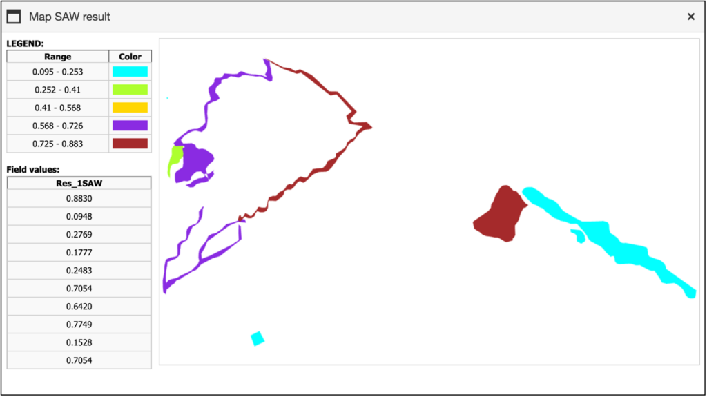
In the MSA context, the interface for “Responses for SAW,” as well as for OWA, WOWA, and TOPSIS, includes an additional button labelled “Map the Score.” Once the global ranking of the spatial object is displayed, the user can click this button to visualize a spatial representation of the scores across different areas. This feature significantly enhances data visualization, making it easier for users to interpret the results within a geographic context. An example of this feature in action for the case study is shown in Figure 37.
2. Ordered Weighted Averaging (OWA)
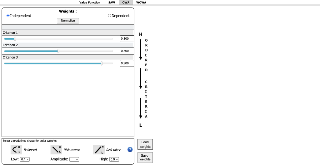
By clicking on the “OWA” Tab Bar, the OWA window appears on the screen. The Ordered Weighted Averaging (OWA) decision rule requires another set of order weights, describing the risk attitude of decision makers (see Methods Handbook).
Unlike the simple weighted average (SAW), where each criterion is directly multiplied by its assigned weight, the ordered weighted averaging (OWA) method ranks the criteria and applies order-specific weights based on their performance position. While OWA still involves multiplying the criterion values by their respective weights and summing the results to calculate the overall performance, the key difference lies in how the criteria are matched with weights (see Methods Handbook for details). In this approach, mDSS first uses the SAW method to determine the initial performance scores of the criteria, considering user-defined importance. These scores are then refined using the OWA procedure for a more nuanced evaluation.
When the number of criteria is large, defining rank-order weights can become tedious. To simplify this process, the user can choose from three predefined functions that automatically compile the values of the order weights. Each function is defined by three parameters, which can be selected according to the risk attitude of the decision-maker the user intends to model. Specifically:
- Risk Averse: the user should select the Low (e.g., 0) and High (e.g., 1) values and and click on the “Risk averse” button. The software assigns the highest weight (e.g., 1) to the criterion with the lowest SAW-weighted performance, and the lowest weight (e.g., 0) to the one with the highest performance. The intermediate weights are linearly distributed. The “Normalise” button rescales the values to sum up to 1.
- Risk Taker: Same procedure, but clicking on the “Risk taker” button, with the software assigning highest weight (e.g., 1) to the criterion with the highest SAW-weighted performance, and the lowest weight (e.g., 0) to the one with the lowest performance.
- Balanced: the user should assign high valiues (e.g., 1) to High and Low and define the Amplitude of the curve with two maxima (ranging from >0 to 1). The software assigns equal weights to the criteria with the highest and lowest SAW-weighted values. The remaining weights are interpolated to follow a parabolic curve, with the curvature defined by the amplitude parameter.
Figure 38 illustrates how the predefined functions are displayed to the user.

For example, if the user wants a linear function characterized by a risk-averse attitude, they should set the parameters to ‘Low,’ ‘High,’ and click on ‘Risk Averse.’ Following this procedure, the mDSS will assign a higher weight to the low-performance indicators and a higher-order weight to the best-performing ones. An example of the software’s output is shown in Figure 39.
If the user desires a more balanced distribution of the order weights, with equal weight for both the best and worst-performing indicators, they can select the same value for both the “Low” and “High” parameters and choose their preferred level of “Amplitude”. Figure 40 provides an example of this scenario.

The weighted criteria values are combined into a single overall performance measure. Once the vector of criteria weights is defined, the “Response for OWA” appears on the right side of the OWA window. The best option is highlighted in yellow, with its score representing 100%. The other options are ranked by their absolute value and displayed as percentages relative to the top-ranked option.
3. Weighted Ordered weighted averaging (WOWA)
By clicking on the “WOWA” tab, the WOWA window will appear on the screen and will look exactly like the OWA window. The Weighted Ordered Weighted Averaging (WOWA) method shares certain mechanisms with OWA and can be considered a generalization of it. The main difference between OWA and WOWA is that while OWA applies double weighting to the criteria performance, WOWA uses a new set of weighted order weights. This new set is derived from the input order weights and the cumulative distribution of the importance weights (see the Methods Handbook for more details).
The method and functions for inserting the vector of order weights into the WOWA window are identical to those used for the OWA window. Once the vector of criteria weights is defined, the “Response for WOWA” will appear on the right side of the WOWA window. The best option is highlighted in yellow, with its score representing 100%. The other options are ranked by their absolute value and displayed as percentages relative to the top-ranked option.
4. TOPSIS
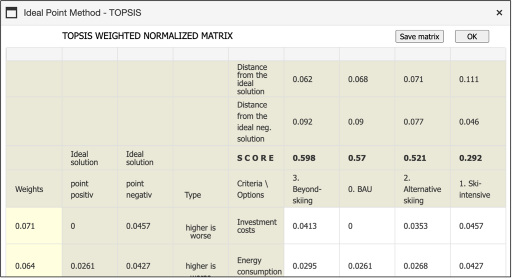
When the TOPSIS method is selected in the Analysis Matrix window, the TOPSIS bar becomes active, and the TOPSIS window appears. The Technique for Order Preference by Similarity to Ideal Solution (TOPSIS) identifies the option that is closest to the positive ideal solution and farthest from the negative ideal solution as the best. Both ideal solutions are defined by the extreme values of the indicators. Since these ideal solutions are theoretical and represent unattainable states, the distance of the real options from both the positive and negative ideal solutions is combined to make the final decision
The TOPSIS window contains several elements:
- a data table in the central area with a white background, displaying the standardized and weighted outcomes for each option;
- the ideal solutions (the best and worst values for each criterion/row) located to the left of the data table;
- the current weights displayed in the first column to the left of the frame.
The calculated Euclidean distances from each option (column) to the ideal solutions are displayed at the top of the table. The aggregated measure of both distances is shown below and forms the basis for ranking the options. The weighted criteria values are combined into a single overall performance measure. An example of the TOPSIS window for the case study is reported in Figure 41. The user can save the outcome by clicking on “Save the matrix”.
Once the vector of criteria weights is defined, and the user selects “Ok”, the “Response for TOPSIS” decision rule appears on the right side of the TOPSIS window. The best option is highlighted in yellow and has a score of 100%. The other options are ranked as percentages relative to the top position.
Sensitivity Analysis and Sustainability
After obtaining the ranking using the SAW, OWA, or WOWA methods, mDSS enables users to perform a sensitivity analysis and access graphical outputs to explore the different dimensions of sustainability for the various options. This section outlines the available tools and visualizations, which can be accessed by clicking the following buttons:
- Sensitivity Analysis
- The Sustainability Chart
- The Sustainability Ranking Chart
- The Ranking Histogram
1. Sensitivity Analysis
The mDSS implements two different methods to perform the sensitivity analysis: the Most Critical Criterion and the Tornado Diagram. After clicking on the button “Sensitivity Analysis”, the user will see a window similar to the one reported in Figure 42.
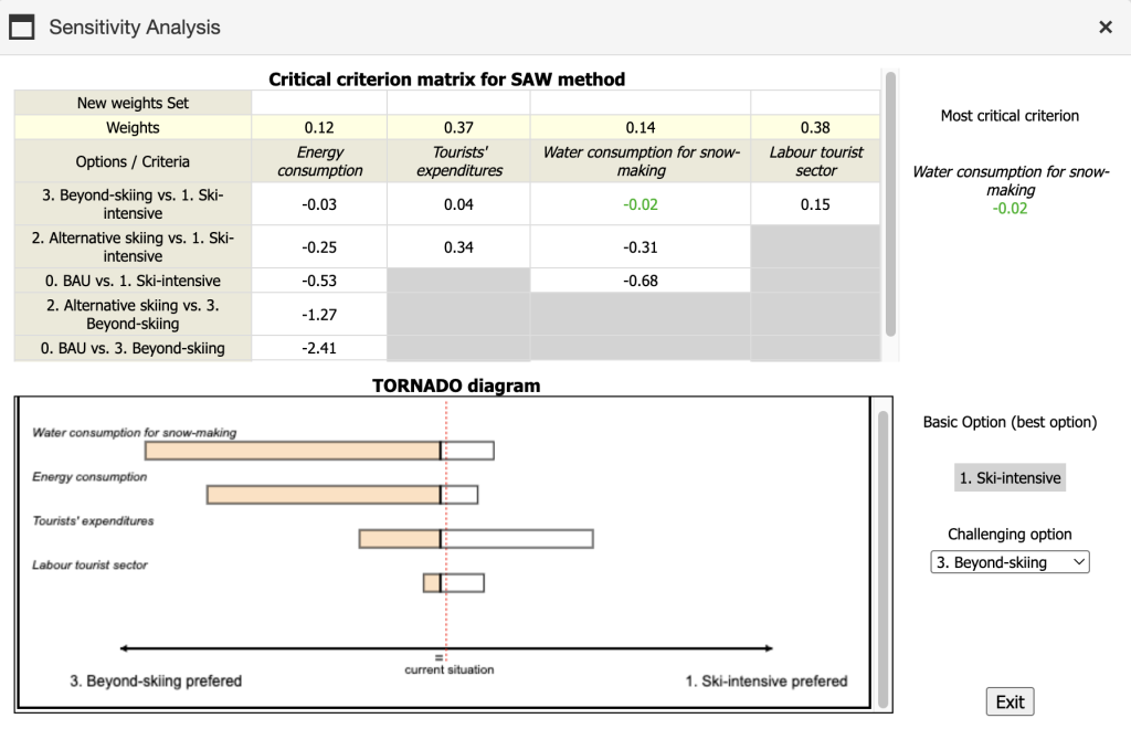
In the example proposed in Figure 42, considering three options and four criteria, the criterion “Water consumption for snow-making” is identified as the most critical criterion. Specifically, it requires the smallest relative change in input weight (in absolute terms) to alter the ranking between two options—in this case, between “3. Beyond-skiing” and “1. Ski-intensive.” In this case, the interpretation is that reducing the weight of the criterion “Water consumption for snow-making” by 2% makes the ranking scores of the two options equal. The table on the left side of the window displays the required relative variation in weight for each criterion and each pair of options. The smallest value, associated with the most critical criterion, is highlighted in green both in the table on the left side and in the upper-right corner of the window.
The Tornado diagram provides a graphical visualization of how sensitive the ranking between two options is to changes in the weights of individual criteria. The options compared are the Basic option (ranked first in the initial analysis) and the Challenging option (selected from the remaining alternatives). In the example shown in Figure 42, these are, respectively, “1. Ski-intensive” and “3. Beyond-skiing.”
The x-axis represents the difference between the ranking scores of the two options across varying levels of criterion weight. The dotted red line indicates the baseline difference observed in the initial ranking (i.e., the current situation). The bold vertical line marks the point where the difference between the two options becomes zero, meaning the user would be indifferent between the two alternatives. The colored section of each bar represents the range of criterion weights where the Challenging option outperforms the Basic option.
To build the diagram, mDSS varies the weight of each criterion individually from 0 to 1, recording the corresponding differences in the ranking scores between the two options. This process is repeated for all criteria. The criteria are then ordered from top to bottom based on their influence on the ranking difference: the greater the influence, the longer the bar and the higher its position in the graph. This creates the characteristic “tornado” shape. For instance, in Figure 42, the criterion “Water consumption for snow-making” produces the largest change in the ranking score difference as its weight varies from 0 to 1. Therefore, it is considered the most influential criterion for the comparison between the two options, and it is represented by the longest bar. Moreover, the graph in the example also shows that there is a value of the weight at which the ranking of the two options is reversed. If a criterion has a bar that is entirely white, it means that no value of the criterion’s weight, when changed alone, can alter the ranking between the two options.ons. Overall, the Tornado diagram offers a quick and intuitive graphical insight into which criteria have the greatest potential to alter the ranking between the two alternatives.
For further details on the sensitivity analysis methods implemented in mDSS, please refer to the Handbook of Methods.
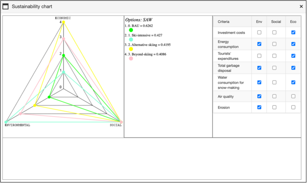
2. The Sustainability Chart
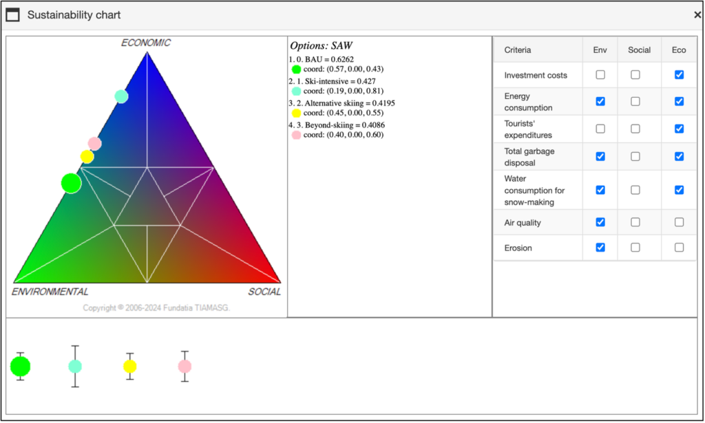
In all the methods supported by mDSS the balance of alternative options across the three pillars of sustainability—Environment, Society, and Economy—can be assessed visually. By clicking the “Sustainability Chart” button, users can aggregate the evaluation criteria into three macro categories based on their nature: environmental, social, and economic. These categories can be defined either in the Indicators window or directly in the sustainability analysis window. Figure 43 illustrates an example of the Sustainability Chart related to the case study.
The weights for each macro criterion are summed, and their relative importance is displayed in a triangle diagram. If the three macro criteria have equal weights, the performance of the option is represented at the centre of the triangle. A position closer to one of the triangle’s corners indicates that the corresponding macro criterion carries more weight than the others. This chart provides a way to evaluate how balanced the various options are across the three pillars of sustainable development, without factoring in their overall performance or ranking.
At the bottom of the screen, coloured circles and black lines are shown. The circles represent the different options, with the area of each circle proportional to its overall performance score. The length of the black lines represents the variability in the values within the evaluation model (EM). A longer line indicates a broader range of variability in the corresponding score, which suggests a greater compensatory effect.
3. The Sustainability Ranking Chart
The “Sustainability Ranking Chart” serves a similar purpose but offers a more intuitive and detailed visualisation of how the options rank across the three key dimensions. Each axis represents the ranking of an option based on its performance in a specific dimension. For instance, in the “Environmental” dimension, the option with the highest score in the environmental indicators will be ranked first, followed by others in descending order. The points representing each option across the three dimensions are then connected by lines, forming a triangle. This triangular shape, generated by the mDSS tool, effectively illustrates the relationships and comparative standings of the options in a clear and cohesive manner. Figure 44 illustrates an example of the “Sustainability Ranking Chart” related to the case study.
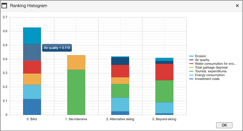
4. The Ranking Histogram
By clicking the “Ranking Histogram” button, a histogram will be displayed, providing a comprehensive view of the total score for each alternative option. In addition to the overall score, the histogram breaks down the contribution of each partial score to the total. These partial scores represent the performance of each alternative option on individual criteria. To view these partial scores, users can hover the cursor on the corresponding criterion’s shape in the graph. The partial scores are calculated based on the standardised indicator values and the weights assigned to each criterion, offering a clear understanding of how each criterion influences the final ranking. Figure 45 illustrates an example of the “Ranking Histogram” related to the case study.