
1 BASIC STEPS OF MCA
Figure 1 shows the basic steps of multicriteria decision analysis as implemented in the mDSS. The decision process starts with problem structuring, during which the problem to be solved is explored, and available information is collected. The possible options – responses in terms of the DPSIR framework – are defined, and criteria aiming at evaluation of their performance are identified. In the next step, the options’ performance in terms of the criteria scores is modeled. As a result, a matrix – called analysis matrix – is constructed. The analysis matrix contains the performance of the raw options using different criteria scales.
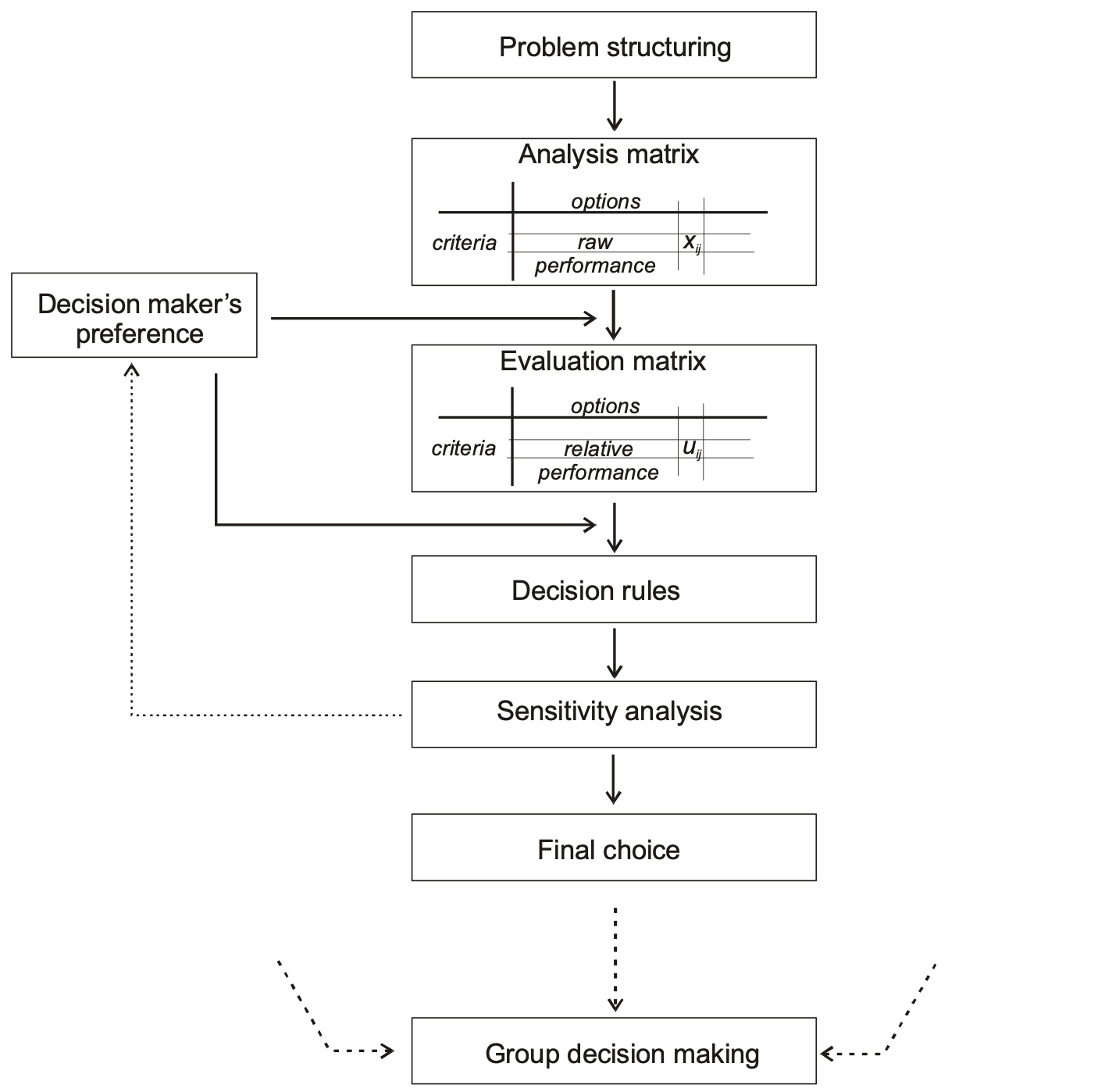
Before any aggregation may start, the options’ performance with regard to different criteria has to be made comparable. During the standardization procedures, or at least by applying a value function, the scores are transformed to values on a uniform scale. Since a simple standardization allows only the transformation of a given value range to a standardized one [0,1], the value function includes human judgments in the mathematical transformation. A value function translates the performance of an option into a value score, which represents the degree to which a decision objective is matched.
Since the main aim of a multicriteria decision analysis is to reduce multiple option performances into a single value to facilitate the ranking process, the heart piece of any MCA decision rule is an aggregation procedure. The large quantity of known decision rules differ in the way the multiple options performance is aggregated into a single value. There is no single method that is universally suitable for any kind of decision problem, the decision maker has to choose the method which best corresponds with his purpose. Finally, a sensitivity analysis examines how robust the final choice is to even a small change in the preferences expressed by the decision maker.
In a situation where there are several decision makers involved in the decision process, the individual choices are to be compared and an option is to be chosen, which represents the group compromise decision.
2 GENERATING THE ANALYSIS MATRIX
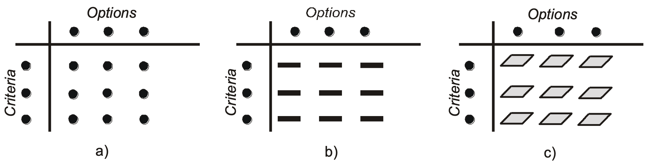
The analysis matrix (M x N: M options and N criteria) is to be built from the environmental indicators identified in the conceptual phase. The cells of the matrix relate to the option-criterion pairs and contain the outcomes or consequences for a set of options and a set of evaluation criteria.
In spatial decision-making, the options are a collection of points, lines, and areal objects with associated attributes. The decision outcomes, as in figure 2b-c, may have spatial extensions. For example, in the case of two-dimension a spatially extended decision outcomes (figure 2c), a cell of the decision matrix corresponds to a map, which contains the spatially distributed consequences of an option with regards to a criterion. Different to the case of non-dimensional (value- or point-like outcomes, figure 2a) consequences, an additional aggregation must be done.
3 STANDARDISING THE ANALYSIS MATRIX
During standardization, criterion values expressed in different measurement units are transformed into a common scale to enable comparison. One possible method is the linear scale transformation, also known as the “score range method”. The method doesn’t maintain the relative order of magnitude but scales the raw options’ scores precisely in the interval [0,1] (formulas 1-2).
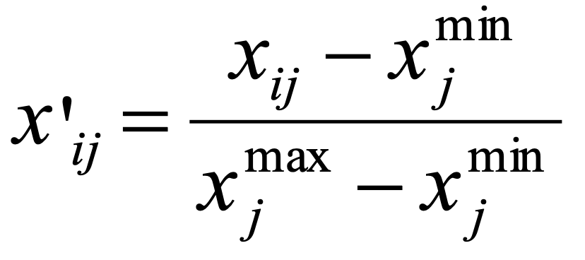
for a criterion to be maximized
1.
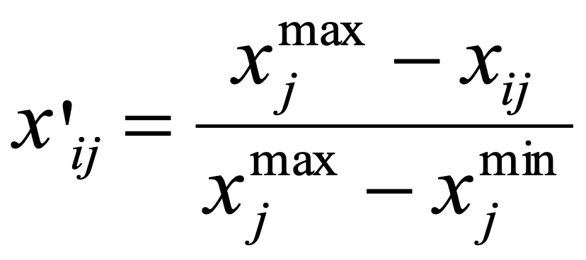
for a criterion to be minimized
2.
The TOPSIS decision rule uses vector normalization (formula 3.). This method has a particular property of producing vectors (the rows of the decision matrix) with the same Euclidean length (equal 1).
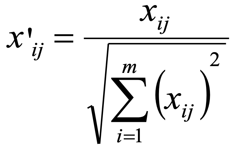
for a criterion to be maximized
3.
4 MODELLING VALUE FUNCTION
The value function is another way of transforming the raw criteria scores into a common scale. However, it allows the preferences of the decision maker to be considered during the transformation.
Decision theory provides a theoretical framework for representing the decision maker’s preferences about the options’ performance. In order to make them more “computational”, the preferences are mapped by the value/utility function (u). A value/utility1 function maps the preference about two options a and b (a ≻ b : a is preferred b) in a numerical relation u(a) > u(b).
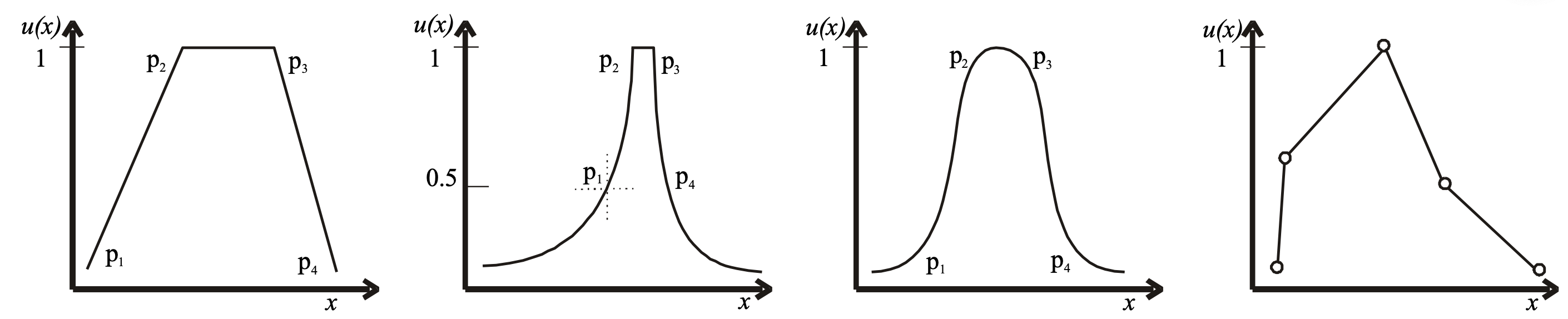
There are several methods for the estimation of the value functions. The mDSS utilizes the direct rating method by which the decision maker immediately assigns a value to each criterion score. The shape of the value function may be selected from the implemented set of value functions, and only their parameters must be specified. In figure 3, some widely used types of value functions are shown. The mDSS supports the piece-linear definition of the value function by the user (figure 3d).
5 MODELLING CRITERIA WEIGHTS
Decision problems involve criteria of varying importance to decision makers. The criterion weights usually provide information about the relative importance of the considered criteria. There are many techniques commonly used for assessing the criterion weights, such as ranking and rating methods, pairwise comparison, and trade-off methods.
Ranking methods use the rank order on the considered criteria. As the rank order describes the importance of the criteria, the information describing them (rank number ri) is used for generating numerical weights.
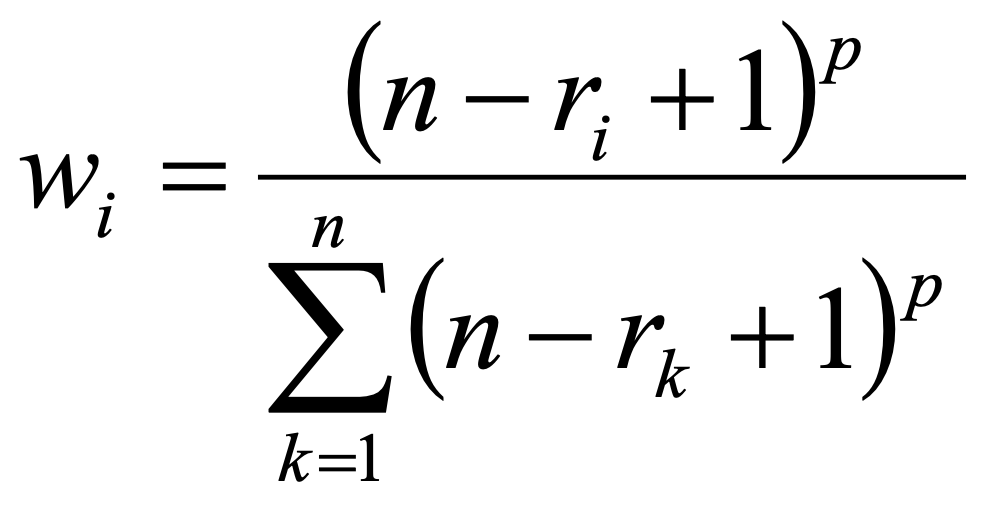
n … number of criteria
ri … rank number of criterion i
p … parameter describing the distribution of the weights
3.
The parameter p may be estimated by a decision maker through interactive scrolling (as in Table 1) or by using predefined formulas that incorporate the weight of the most important criterion as input from the decision maker. For p = 0 results to equal weights. As p increases, the weights distribution becomes steeper. Table 1 shows the estimated weights for some values of p.
| Parameter p | ||||||||
| Rank | 0 | 0,5 | 1 | 2 | 3 | . | 10 | |
| Most important criterion | 1 | 0,2 | 0,26 | 0,33 | 0,45 | 0,55 | . | 0,89 |
| . | 2 | 0,2 | 0,23 | 0,26 | 0,29 | 0,28 | . | 0,09 |
| . | 3 | 0,2 | 0,2 | 0,2 | 0,16 | 0,12 | . | 0 |
| . | 4 | 0,2 | 0,16 | 0,13 | 0,07 | 0,03 | . | 0 |
| Less important criterion | 5 | 0,2 | 0,11 | 0,06 | 0,01 | 0 | . | 0 |
| Sum | 1 | 1 | 1 | 1 | 1 | . | 1 | |
Table 1. The behaviour of the generated numerical weights depends on the parameter p of the rank component method
Pairwise comparison method was developed by Saaty (1980, quoted by Malczewski 1999) in the context of his decision rule called Analytic Hierarchy Process. The method involves pairwise comparisons to create a ratio matrix. Through the normalization of the pairwise comparison matrix, the weights are determined.
The method uses an underlying scale with values, from 1 to 9 for example, to describe the relative preferences for two criteria. The result of the pairwise comparisons is a reciprocal quadratic matrix (Table 2b). Table 2a presents the scale for pairwise comparison, while Table 2b shows the pairwise comparison matrix between four criteria (C1–C4).
| 1 | Equal importance |
| 3 | Moderate importance |
| 5 | Strong importance |
| 7 | Very strong importance |
| 9 | Extreme importance |
| 2, 4, 6, 8 | Intermediate values between two adjacent judgments |
| C1 | C2 | C3 | C4 | |
| C1 | 1 | 4 | 7 | 5 |
| C2 | 1/4 | 1 | 1/3 | 9 |
| C3 | 1/7 | 3 | 1 | 5 |
| C4 | 1/5 | 1/9 | 1/5 | 1 |
Using the pairwise comparison matrix A ∈ ℝⁿˣⁿ the weights wj may be determined as below:
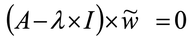
- Estimate the maximum eigenvalue λmax of the comparison matrix, which fulfils formula 5:
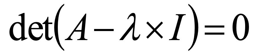
5.
- Determine the solution w̃ as in formula 6:
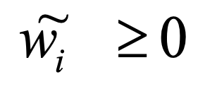
6.
- Normalize the w̃ by formula 7
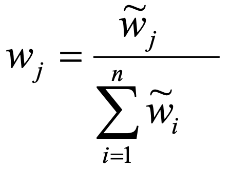
7.
After the weights have been determined, the consistency of pairwise comparison must be evaluated. The procedure of the consistency test may be found in the Annex.
The Saaty method deals with the consistency of the pairwise comparison matrix. A consistent matrix means for example if the decision maker says a criterion x is equally important to another criterion y (so the comparison matrix will contain value of axy = 1= ayx), and the criterion y is absolutely more important as an criterion w (ayw = 9; awy = 1/9); then the criterion x should also be absolutely more important than the criterion w (axw = 9; awx = 1/9). Unfortunately, the decision maker is often not able to express consistent preferences in the case of multiple criteria. Saaty’s method measures the inconsistency of the pairwise comparison matrix and sets a consistency threshold which should not be exceeded (for details about the consistency of pairwise comparison matrix, see the Annex).
Hierarchical Weighting Method, Saaty (1980), generalizes the Pairwise Comparison Method by introducing a hierarchical structure into the evaluation process. This generalization extends the application of pairwise comparisons to multiple levels of criteria, allowing for a comprehensive and organized assessment of their relative importance. The steps are:
- Define the hierarchy: Establish the main criteria and sub-criteria (if any) relevant to the decision problem.
- Assign weights: Determine the relative importance of each criterion at each level of the hierarchy.
- Aggregate weights: Combine these weights to calculate the overall weight of each criterion in the context of the decision problem.
Following the example in Table 2, suppose that criteria C1 and C2 can be grouped into the broader set G1 and C3 and C4 into the broader set G2. The Hierarchical Weighting Method evaluates the weight to assign to each criterion ( C1, C2, C3, C4) considering also the result of the Pairwise Comparison Method with respect to G1 and G2. In a situation where:
- the Pairwise Comparisons shows that C1 and C2 have the same relative importance
- the Pairwise Comparisons shows that C3 and C4 have the same relative importance
- the Pairwise Comparisons between G1 and G2 shows that G1 the has twice the importance of G2
The final weights for the criteria ( C1, C2, C3, C4) would be (0.33, 0.33, 0.165, 0.165).
Swing weights are assigned through the supposed increase of each criterion’s performance from the worst to the best value. The criterion that represents the highest boost to the total options’ performance is assigned a value of 100, all the other criteria are compared respectively to this criterion. As Belton and Stewart (2002) put it, “If a swing from worst to best on the most highly weighted criterion is assigned a value of 100, what is the relative value of a swing from worst to best on the second-ranked criterion”?
Simos weights, initially developed by Simos (1990a,1990b), are defined following the decision maker’s (DM) preferences regarding the ranking of criteria and the relative importance of each position in the ranking. Originally conceived as a visual method, this approach uses numbered cards to establish the ranking of criteria (e.g., position 1, position 2, etc.) and blank cards to represent the relative importance between these ranked positions. The number of blank cards placed between two numbered positions indicates the degree of difference in importance between them; more blank cards suggest a greater disparity in importance. Various modifications of this method have emerged, maintaining the original simplicity and intuitive nature. In mDSS, weights are determined based on the criteria’s importance ranking and the relative importance assigned between the highest and lowest-ranked criteria.
- The term value function is used in the context of decision under certainty. The utility function refers to the situation under risk consideration, i.e. when the outcomes are associated with a probability. ↩︎