Sensitivity analysis (SA) is an important task in multicriteria decision-making: it looks at how robust (or weak) the final decision is, in the case that even a slight change in the decision outcomes or previously expressed preferences is made. Sometimes the sensitivity analysis is distinguished from a robustness analysis: while the sensitivity analysis is assumed as the analysis of the effects of changing data and model parameters in a constrained vicinity to a base solution, the robustness analysis is considered a systematic analysis of a large set of variations which are plausible in the decision problem context.
1 INTRODUCTION
Sensitivity analysis deals with the investigation of potential changes and errors and their impacts on the results of underlying models. Sensitivity analysis, applied post-hoc to decision models, deals with uncertainties related to the decision outcomes and/or to the preferential judgements (i.e. value function and criterion weights). The objective is to find out how the options ranking changes by any modification made on the decision models. While the impact of uncertainties on the decision outcomes is mostly analysed by statistical modelling and simulation, the preferential judgements are object of uncertainty during the modelling of weights and value function. However, SA provides neither a explicit probabilistic measure of the risk to make a wrong decision nor an explicit treatment of the risk attitude of the DM.
Sensitivity analysis may be used for wide range of different uses (for detail see Pannell 1997). The SA methods are useful within (i) decision making for identifying critical value/criterion, testing robustness and riskiness of decision; (ii) communication for increasing credibility and confidence; and (iii) modelling process for better understanding of input-output relationship and for understanding the model needs and restrictions.
Sensitivity analysis approaches differ in the level that they address: (i) approaches targeted to local level consider only the immediate neighbourship of a given starting point (e.g. a previously identified optimal solution of a decision problem); while (ii) the approaches working on a global level vary all input parameters over their range of uncertainty. At the same time one or more parameter may be considered to vary. By a single parameter test all other parameters are held fixed. This is a common approach that is used, although the interactions between two or many parameters are ignored and their combined impact is not analysed. On the other side, multi-parameter tests are computationally very complex and thus less practical.
Performing the sensitivity analysis may be a complex undertaking. Considering just a simple example with 5 options and 5 criteria: the simulation of the criterion weight taking into account only 20 different values for a weight (sampling step 0,05) would encompasses 4151 calculations of overall preference function producing 4151 feasible ranking vectors. Additionally, the search for the feasible weights’ combination from all 3.200.000 ones is also considerable.
A suitable SA depends on the decision rules chosen for the preferences aggregation. While the decision rules discussed for implementation in the mDSS are mostly based on criteria weights, the main concern of the sensitivity analysis will be oriented to the uncertainty addressing the criterion weights.
The mDSS utilises two approaches for SA:
- most critical criterion: identifying the criterion for which the smallest change of current weight may alter the existing ranking of options; and
- tornado diagram: graphically comparing the chosen option with any other one and showing ranges within which the parameters may vary.
1.1 MOST CRITICAL CRITERION
This method developed by (Triantaphyllou 2000) considers the most critical criterion to be the one which requires the minimal amount of change in the current value of its weight in order to change the options’ rank order. Using this method, the user may directly test if the minimal change in criteria weights which leads to the final rank disturbance is within or outside his confidence range.
The method distinguishes two rank order changes:
- the top critical criterion is that one which changes the best ranked option (T method).
- any critical criterion is that one which changes ranking of any options (A method).
The algorithm to estimate the critical criterion encompasses following steps:
1.1 List all possible changes in options’ rank order caused by modification of criteria weights (e.g. how much must change the weight wi in order to change the rank order between the first two options). There are only
(n × m (m-1)) / 2
changes in rank order possible (with n… number of criteria; and m.. number of options).
In case of three options and two criteria: there are three possible rank order changes which may be caused by changes in two criteria – 2 * 3 * 2 / 2 = 6
| c1 | c2 | |
| a2 ↑ ↓ a1 | 1 | 2 |
| a3 ↑ ↓ a1 | 3 | 4 |
| a3 ↑ ↓ a2 | 5 | 6 |
1.2 For each change of options’ rank order calculate the difference of total options’ performance
| ΔP | |
| a2 ↑ ↓ a1 | (P2 – P1) |
| a3 ↑ ↓ a1 | (P3 – P1) |
| a3 ↑ ↓ a2 | (P3 – P2) |
(Pi is obtained as result of decision rule from the choice phase, aggregation result)
1.3 For each rank change and for each criterion calculate difference between the options’ performance.
| c1 | . | cn | |
| a2 ↑ ↓ a1 | a21 – a11 | . | a2n – a1n |
| a3 ↑ ↓ a1 | a21 – a11 | . | a3n – a1n |
| . . . | . . . | . | … |
| am ↑ ↓ am-1 | am,1 – am-1,1 | . | am-1,n – am, n |
(aij is the corresponding value from the evaluation matrix, i.e. standardised and weighted option’s score)
1.4 Calculate a new matrix dividing the cell values of the matrices created in step 2 and 3.
| c1 | . | cn | |
| a2 ↑ ↓ a1 | (P2 – P1) / (a21 – a11) | . | (P2 – P1) / (a2n – a1n) |
| a3 ↑ ↓ a1 | (P3 – P1)/ (a21 – a11) | . | (P3 – P1)/ (a3n – a1n) |
| . . . | . . . | . | … |
| am ↑ ↓ am-1 | (Pm – Pm-1) / (am,1 – am-1,1) | . | (Pm – Pm-1) / (am-1,n – am, n) |
1.5 Exclude unfeasible weights changes
The unfeasible solution (no changes in weights are able to change the rank order) should be excluded from consideration. The value of the previous matrix are feasible if there are less then the criteria weights (wk) indicated by user and used for aggregation in the choice phase.
(Pj – Pi)/ (ajk – aik) ≤ wk
where i and j indicate two options (best option ≤ i < j ≤ worst solution) and k indicate a criterion.
1.6 The remaining feasible solutions represent changes in the corresponding weights in order to reverse the option ranking. The rows minimal (absolute) value indicates the critical criterion for a given change in rank and the minimal feasible value in the whole matrix indicates the critical criterion for any changes in options’ rank order. To obtain the critical criterion for top rank changes the minimal value in the first (m – 1) rows is to be found.
| c1 | . | cn | ||
| A2 ↑ ↓ a1 | minimal value indicate critical criterion to reverse the rank order between a2 – a1 | minimal value indicate critical criterion to reverse the rank order between the best ranked (a1) and any other option | ||
| A3 ↑ ↓ a1 | minimal value indicate critical criterion to reverse the rank order between any options’ pair | |||
| . . . | ||||
| am ↑ ↓ am-1 | ||||
| Considering the following decision matrix (left) producing the aggregated options performances as in the column right | |||||||||||||||
| c1 | c2 | c3 | |||||||||||||
| wi | 0,33 | 0,33 | 0,33 | Pi | |||||||||||
| a1 | 0.2 | 1 | 0.4 | 0.528 | |||||||||||
| a2 | 0.5 | 0.3 | 0.4 | 0.5*0.33 + 0.3*0.33 + 0.4*0.33= 0.396 | |||||||||||
| After applying a SAW aggregation method the option a1 is preferred. The goal of the SA is to find out, which criterion weights is most sensible for the final ranking and how much is it to be changed in order to reverse the options ranking. Calculation of the differences in options performances (a2i – a1i) – left; right – calculation of difference in options’ performance (⊗P) | |||||||||||||||
| c1 | c2 | c3 | ΔP | ||||||||||||
| a2 ↑ ↓ a1 | 0.5 – 0.2 =0.3 | 0.3 – 1 = – 0.7 | 0.4 – 0.4 = 0 | 0.396 – 0.528 = – 0.132 | |||||||||||
| Calculation of the (P2 – P1) / (a2i – a1i) | |||||||||||||||
| c1 | c2 | c3 | |||||||||||||
| a2 ↑ ↓ a1 | – 0,132/0.3 = – 0.44 | – 0,132/ – 0.7 = 0.188 | ∅ | ||||||||||||
| Identifying the most critical criterion and the magnitude of the change of its weight | |||||||||||||||
| c1 | c2 | c3 | |||||||||||||
| a2 ↑ ↓ a1 | – 0.44 | 0.19 | ∅ | ||||||||||||
| → Consistency check – change of both criteria weights may cause rank reverse because both value above are less then the current criteria weights → Critical criterion = c2 because |0.188| < |-0.44| Calculation of new weight w2′ w2′ = 0.33 – (0.19) = 0.14 Standardisation of new weights (w*) w1* =w1/(w1’+w2+w3)=0.33/0.8 = 0.41 w2* =w2’/ /(w1’+w2+w3) = 0.14/0.8 = 0.18 w3* = w3/(w1’+w2+w3) = 0.33/0.8 = 0.41 Proof: Applying the new weight set the resulting aggregated performances are equal. | |||||||||||||||
| c1 | c2 | C2 | |||||||||||||
| wi | 0,41 | 0,18 | 0,41 | Pi | |||||||||||
| a1 | 0.2 | 1 | 0.4 | 0.42 | |||||||||||
| a2 | 0.5 | 0.3 | 0.4 | 0.42 | |||||||||||
1.2 TORNADO DIAGRAM
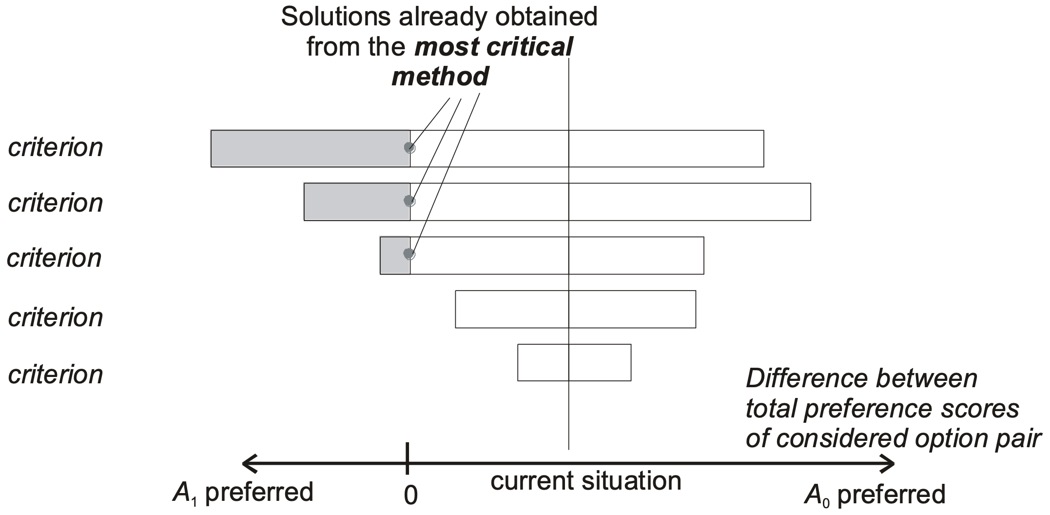
The Tornado diagram provides a graphical visualization of how sensitive the ranking between two options is to changes in the weights of individual criteria. The options compared are the Basic option (ranked first in the initial analysis) and the Challenging option (selected from the remaining alternatives). In Figure 5, these options are, respectively, “A0” and “A1”.
The x-axis represents the difference in ranking scores between the two options, evaluated across varying levels of criterion weight, which range from 0 to 1. The black line shows the baseline difference observed in the initial ranking (i.e., the current situation). Grey points indicate where the difference becomes zero, meaning the user would be indifferent between the two options. The coloured portion of each bar highlights the range of weights where the Challenging option outperforms the Basic option.
This format helps identify which criteria have the greatest influence on the outcome: the longer the criterion bar, the greater its potential impact on the final result when its weight is varied across its full range. In the graphical visualization, criteria are ordered in descending order by bar length, creating a tornado-like shape that gives this sensitivity analysis method its name.