
Decision rules aggregate partial preferences describing individual criteria in a global preference and then rank the options. The decision rules chosen for implementation in the mDSS include (i) simple additive weighting (SAW), (ii) order weighting average (OWA), (iii) weighted order weighting average (WOWA) and (iv) an ideal point method (TOPSIS).
These decision rules cover a wide range of decision situations and may be chosen by the decision maker according to the specifics of a given decision problem.
- SAW is one of the most popular decision methods because of its simplicity. It assumes additive aggregation of decision outcomes, which is controlled by weights expressing the importance of criteria.
- OWA is being used because of its potential to control the trade-off level between criteria and to consider the risk behaviour of the decision makers.
- WOWA is a more sophisticated variant of OWA, based on order weights defined as functions of importance weights. This approach effectively resolves the issue of double weighting of criteria performance inherent in OWA, resulting in a more precise and balanced aggregation of decision criteria.
- Ideal point methods like TOPSIS order a set of options on the basis of their separation from the ideal solutions. The option that is closest to the ideal positive solution and furthest from the negative ideal solution is the best one.
1 SIMPLE ADDITIVE WEIGHTING (SAW)
Simple additive weighting is a popular decision rule because of its simplicity. It uses the additive aggregation of the criteria outcomes (Formula 8).
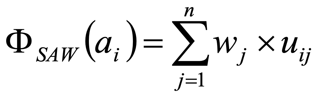
wj .. criterion weights
8.
| Considering a simple example of two options and three criteria: | |||||
| wi | a1 | a2 | |||
| c1 | 0.4 | 0.2 | 0.8 | ||
| c2 | 0.4 | 0.5 | 0.11 | ||
| c3 | 0.2 | 0.9 | 0.25 | ||
| The SAW aggregation is performed as follows: ΦSAW(a1) = 0.2 * w1 + 0.5 * w2 + 0.9 * w3 = 0.2 * 0.4 + 0.5 * 0.4 + 0.9 * 0.2 = 0.46 ΦSAW(a2) = 0.8 * w1 + 0.11 * w2 + 0.25 * w3 = 0.8 * 0.4 + 0.11 * 0.4 + 0.25 * 0.2 = 0.414 Since Φ(a1) = 0.46 > 0.414 = Φ(a2), the option a1 is preferred – a1 a2 | |||||
2 ORDER WEIGHTING AVERAGE (OWA)
The Ordered Weighted Averaging (OWA) operator provides continuous fuzzy aggregation operations between the fuzzy intersection (MIN or AND) and union (MAX or OR), with a weighted linear combination falling midway in between. It adopts the logic of (Yager) and can achieve continuous control over the operator’s degree of ANDORness and the degree of tradeoff between criteria.
The criteria are weighted on the basis of their rank order rather than their inherent qualities. By so doing the weights – called order weights – are applied to the criteria according to the rank order across their scores. For a given option, the order weight ow1 is assigned to the criterion with the lowest score, order weight ow2 to the criterion with next higher-ranked scores, and so on. Consequently, an order weight owi may be assigned to different criteria by two options o1 and o2, depending on the rank order of their scores.
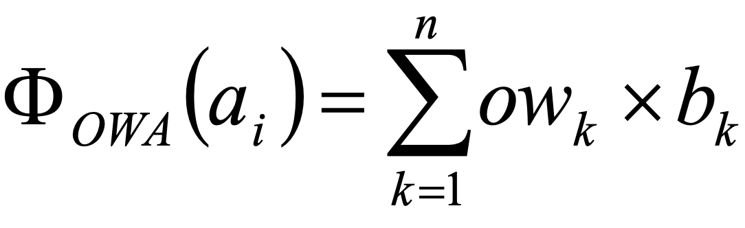
9.
where bk denotes the k-th lowest score of the options i (uij)
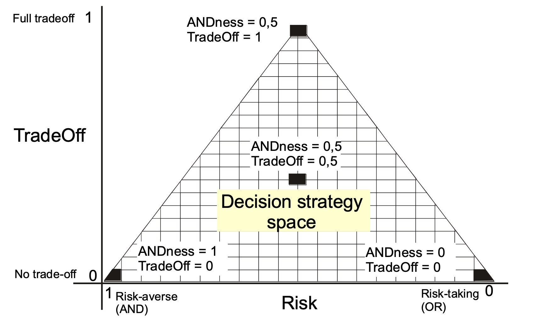
Trade-off means that a very low score in one criterion may not be compensated with a very high score in another one. The SAW decision rule described in chapter 2.6.1 allows full trade-off. The MAXIMAX decision rule, in which the decision maker selects the option with the maximal scores in the best criterion, and the MAXIMIN rule, by which the option with the best scores in the worst criterion is selected, don’t allow any trade-off as the decision is made according only to one criterion.
OWA may be characterised as a control allowing an aggregation between the MAXIMAX, MAXIMIN and SAW extremes. In the case of 3 criteria the set of order weights [1, 0, 0] assigns the extreme importance to the lowest criterion score and corresponds to the MAXIMIN rule. The order weights [0, 0, 1] in contrast assign the extreme importance to the largest criterion score and correspond to the MAXIMAX rule. Equally distributed order weights [0.33; 0.33; 0.33] apply some importance to each rank and don’t change the options ranking obtained from the SAW rule.
| Considering two options and three criteria as in the table below | |||||
| a1 | a2 | ||||
| c1 | 0.2 | 0.8 | |||
| c2 | 0.5 | 0.11 | |||
| c3 | 0.9 | 0.25 | |||
| The order weights [ow1 = 0.5; ow2 = 0.2 ; ow3 = 0.3] will be assigned to the criteria for each option as following: | |||||
| a1 | a2 | ||||
| c1 | ow1 | ow3 | |||
| c2 | ow2 | ow1 | |||
| c3 | ow3 | ow2 | |||
| The OWA aggregation is performed according to the previous table: Φ(a1) = 0.2 * ow1 + 0.5 * ow2 + 0.9 * ow3 = 0.2 * 0.5 + 0.5 * 0.2 + 0.9 * 0.3 = 1.4 Φ(a2) = 0.11 * ow1 + 0.25 * ow2 + 0.8 * ow3 = 0.11 * 0.5 + 0.25 * 0.2 + 0.8 * 0.3 = 0.345 Since Φ(a1) = 1.4 > 0.345 = Φ(a2), the option a1 is preferred – a1 ≻ a2 | |||||
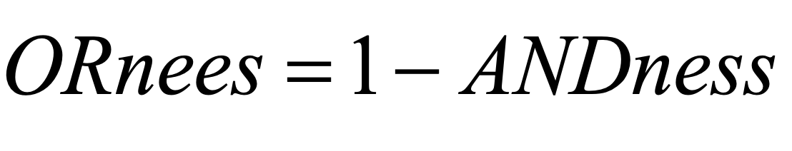
The ANDness, ORness and TRADEOFF characteristics of any particular distribution of the order weights may be calculated using the formulas (10-12).
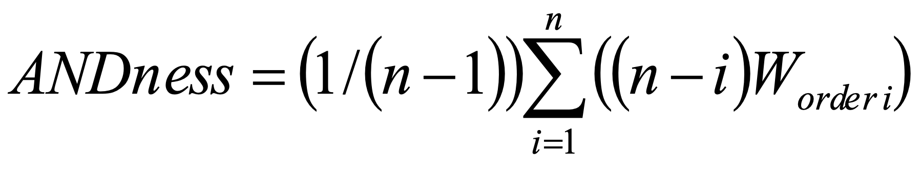
n .. number of criteria
10.
i .. criterion rank order
11.
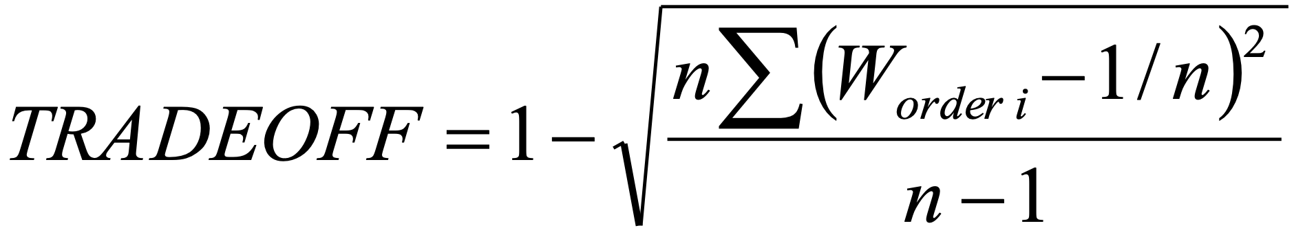
Worder_i .. order weight of i-th criterion
12.
In table 3 these characteristics are calculated for a selected set of order weights.
| Order weights | |||||
| ow1 | ow2 | ow3 | ANDness | TRADEOFF | |
| MAXIMIN = | 1 | 0 | 0 | 1 | 0 |
| 0,9 | 0,1 | 0 | 0,95 | 0,15 | |
| 0,8 | 0,2 | 0 | 0,90 | 0,28 | |
| 0,5 | 0,5 | 0 | 0,75 | 0,50 | |
| 0,5 | 0,3 | 0,2 | 0,65 | 0,74 | |
| 0 | 1 | 0 | 0,50 | 0,00 | |
| 0 | 0,8 | 0,2 | 0,40 | 0,28 | |
| MAXIMAX = | 0 | 0 | 1 | 0,00 | 0,00 |
| SAW = | 0,33 | 0,33 | 0,33 | 0,50 | 1 |
Graphical representation of all possible distributions of order weights is shown in Figure 4.
3 WEIGHTED ORDER WEIGHTING AVERAGE (WOWA)
The WOWA (Weighted Ordered Weighted Averaging) operator is an extension of the OWA (Ordered Weighted Averaging) operator that combines the principles of OWA and weighted averaging in a single framework. mDSS refers to the work of Torra (1997), who introduced a more sophisticated aggregation process capable of capturing both the relative importance of criteria and the sequential order of their corresponding scores. WOWA thus offers a continuous control between extremes, similar to OWA, but with additional flexibility due to the incorporation of explicit criterion weights. It can be thought of as a generalisation of both SAW and OWA, since they can be thought of as special cases of the WOWA operator.
WOWA operates by first assigning a weight to each criterion based on its inherent importance (as determined by the decision maker). Then, it reorders the criteria according to their scores for a given option, just like OWA. Finally, the WOWA operator aggregates the scores by applying both the criterion-specific weights and the order-based weights (order weights). Mathematically, WOWA can be expressed as a function of both the criterion weights and the order weights, allowing for sophisticated trade-offs between criteria. The method provides a flexible decision-making tool that can adapt to various decision contexts by adjusting the degree of trade-off allowed between criteria.
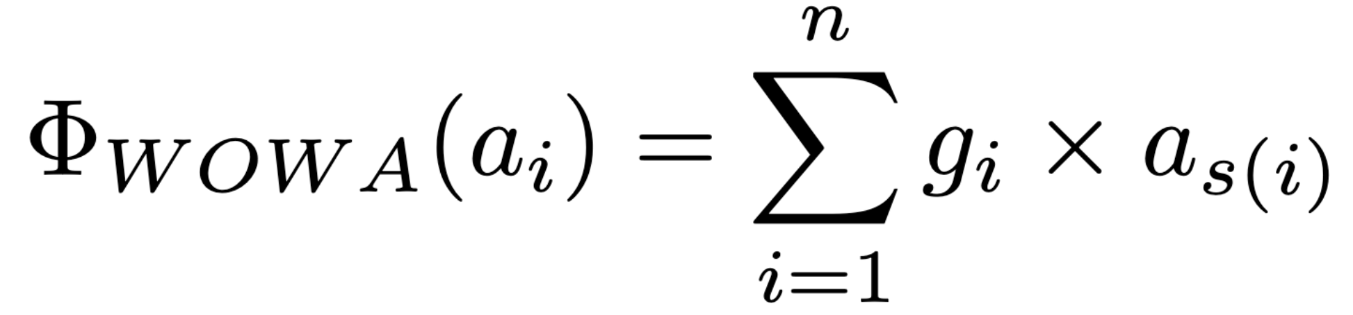
13.
where {s(1),…,s(n)} is a permutation of {1,…,n} such that as(i-1) ≥ as(i) for all i=2,…,n. (i.e., as(i) is the ith largest element in the collection a1,…,an)
The weight gᵢ is defined as
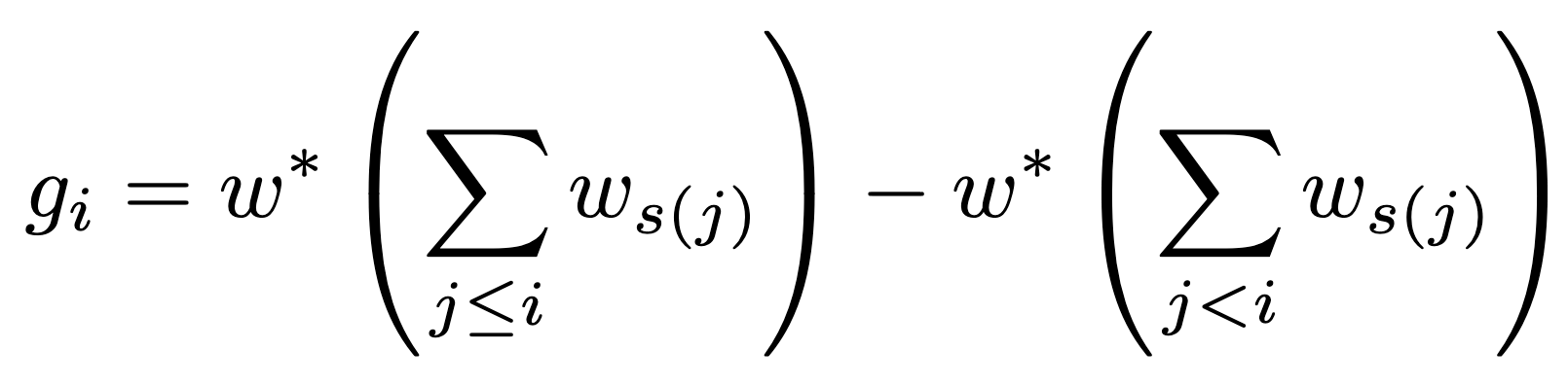
14.
with w* a monotone-increasing function that interpolates the points
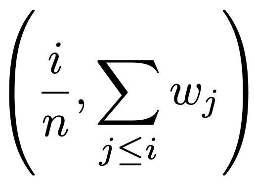
together with the point (0,0).
w* is required to be a straight line when the points can be interpolated in this way. For a comprehensive explanation of the method, refer to Torra (1997).
| Considering two options and three criteria as in the table below | |||||
| a1 | a2 | ||||
| c1 | 0.2 | 0.8 | |||
| c2 | 0.5 | 0.11 | |||
| c3 | 0.9 | 0.25 | |||
| The criteria importance weights assigned by the decision maker are [w1 = 0.2; w2 = 0.5 ; w3 = 0.3]. Ordering the criteria from the less important to the most important, the vector of the cumulative distribution of the importance weights (wi) is T = [0.2; 0.5; 1]. In our example, the criteria importance order is 0.2 (c1) < 0.3 (c3) < 0.5 (c2). Since the vector of the importance weights is only one for each DM, this order will be the same for each of the alternative WOWA score calculations. | |||||
| Starting from a1, the first alternative, the criteria are now ordered following their performance. In our example, the order is 0.2 (c1) < 0.5 (c2) < 0.9 (c3). NOTE: This order can be different for each ai ! Following the performance order, the order weights are assigned to each criterion, just like OWA. In our example, the criteria order weights are [ow1 = 0.4; ow2 = 0.35 ; ow3 = 0.25]. In this case, a greater relevance is given to the lowest criteria performances (risk-averse DM). | |||||
| a1 | a2 | ||||
| c1 | ow1 | ow3 | |||
| c2 | ow2 | ow1 | |||
| c3 | ow3 | ow2 | |||
The cumulative distribution of the WOWA weights (w*) can now be created for each ai. In our example, for a1, the function is designed as a linear interpolation of the points: (0, 0); (⅓; 0.4); (⅔; 0.65); (1; 1). 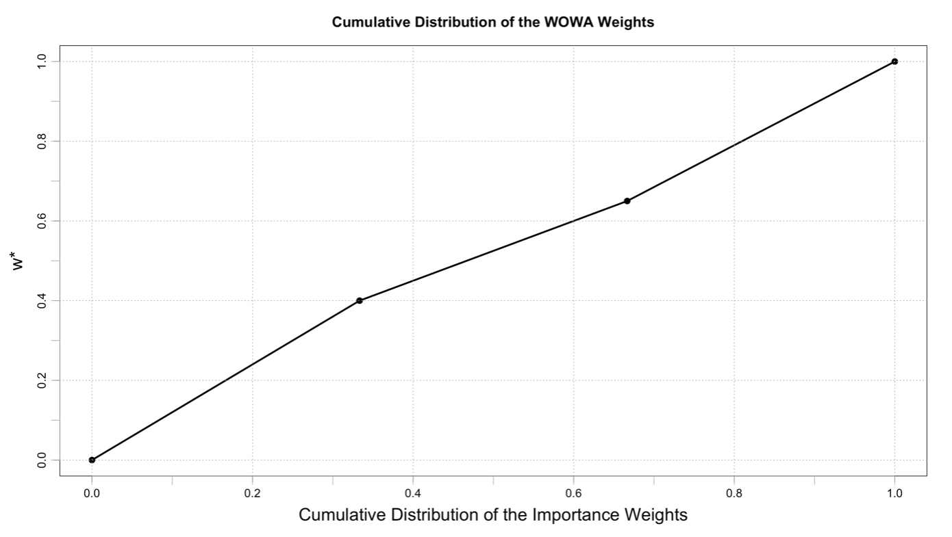 As presented in formula 14, the coordinates for the x-axis are defined by i/n (n = # of the criteria). In our case, the values are: ⅓ ; (⅓ + ⅓) = ⅔; (⅓ + ⅓ + ⅓) = 1. For the y-axis, the coordinates are determined as the cumulative distribution of the order weights, following the importance criteria order defined in the first step. We found that the importance criteria order is 0.2 (c1) < 0.3 (c3) < 0.5 (c2). In the creation of the function, the first criterion to be evaluated must be c1. Since, for a1, the order weight of c1 is ow1 = 0.4, the first point of w*, after (0,0), is (⅓; 0.4). Following the importance order, the second criterion to be evaluated is c3. Since, for a1, the order weight of c3 is ow3 = 0.25, the second point of w* is (⅔; 0.4 + 0.25 = 0.65). The last point of w* is (1, 1) by construction. NOTE: Each ai can have different w* shapes and different WOWA weights for the same criteria! | |||||
| Defined w*, the WOWA weights gi are determined as shown in Formula 14. The input is the vector T = [0.2; 0.5; 1], the cumulative distribution of the importance weights. In our example, for a1: g1 = w*(0.2) = 0.24 g3 = w*(0.5) – w*(0.2) = 0.525 – 0.24 = 0.285 g2 = w*(1) – w*(0.65) = 1- 0.525 = 0.475 | |||||
| The WOWA aggregation is performed according to formula 13: Φ(a1) = 0.2 * g1+ 0.5 * g2 + 0.9 * g3 = 0.2 * 0.24+ 0.5 * 0.475 + 0.9 * 0.285 = 0.542 Following the same reasoning, the same process is applied to a2: Φ(a2) = 0.11 * g1 + 0.25 * g2 + 0.8 * g3 = 0.11 * 0.425 + 0.25 * 0.425 + 0.8 * 0.15 = 0.273 Since Φ(a1) = 0.542 > 0.273 = Φ(a2), the option a1 is preferred – a1 ≻ a2 Note: Each alternative, for each criteria, has different values of gi! | |||||
1.2 IDEAL POINT METHODS (TOPSIS)
Ideal point methods order a set of options on the basis of their separation from the ideal solution. The ideal solution represents an (not achievable and thus only hypothetical) option that consists of the most desirable level of each criterion across the options under consideration. The option that is closest to the ideal point is the best one. The measurement of separation requires distance metrics. The ideal negative solution may be defined in the same way: the best option in this case is characterized by the maximum distance from it. The formulas 15 and 16 show the generalized definition of distance metrics (using weighted Minkowski LP metrics). For p = 1, the rectangular or city distance is calculated. For p = 2 the Euclidean distance is obtained.
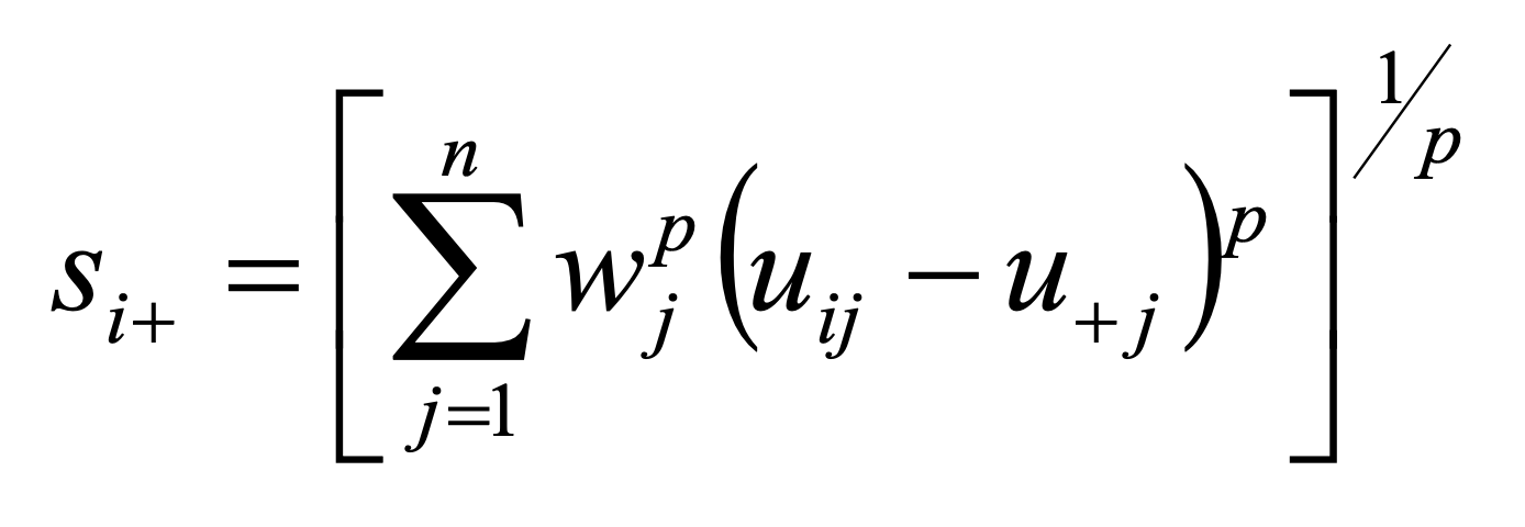
15.
si+ … separation of the ith option from the ideal point
wj … weight assigned to the criterion j
u+j … ideal value for the jth criterion
p … power parameter ranking from 1 to ∞
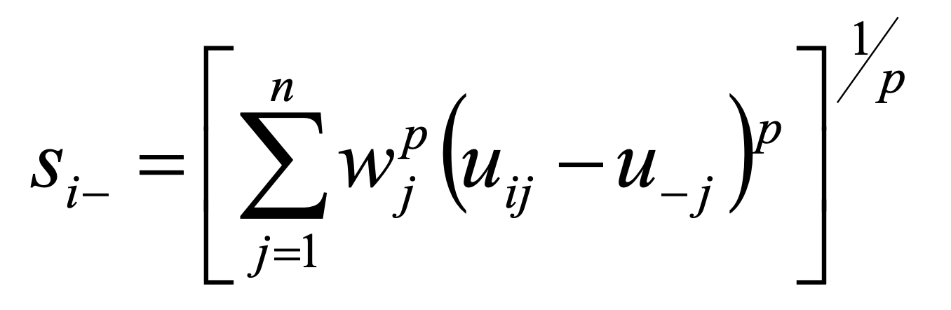
16.
si- … separation of the ith option from the negative ideal point
uj … negative ideal value for the jth criterion
TOPSIS (Technique for Order Preference by Similarity to Ideal Solution) is one of the most popular compromise methods. TOPSIS defines the best option as the one that is closest to the ideal option and farthest away from the negative ideal point. The method requires the cardinal form of the performance of options. The distance from the ideal / negative ideal point is calculated as in Formula 17 and 18.
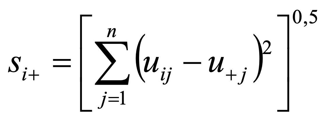
17.
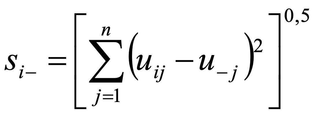
18.
The relative closeness to the ideal solution (ci+), which will be used for the ranking of options, is calculated as in formula 17.
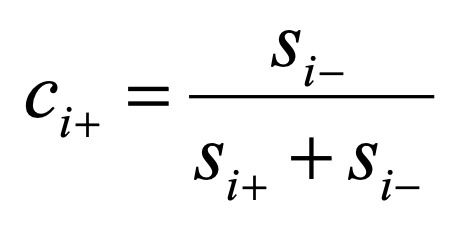
19.
| Considering a simple example of two options and three criteria with already weighted performances | ||||||
| a1 | a2 | ideal positive solution | ideal negative solution | |||
| C1 | 0.08 | 0.32 | 0.32 | 0.08 | ||
| C2 | 0.2 | 0.044 | 0.2 | 0.044 | ||
| C3 | 0.18 | 0.05 | 0.18 | 0.05 | ||
| The distances from the positive and negative ideal solutions as well as the final aggregation according to the formula 17 is performed as following: | ||||||
| a1 | a2 | |||||
| si+ | 0.24 | 0.20 | ||||
| si- | 0.20 | 0.24 | ||||
| ci+ | 0.46 | 0.54 | ||||
| For example si+(a1) = ((0.08 – 0.32)^2 + (0.2 – 0.2)^2 + (0.18 – 0.18)^2)^0.5 = 0.24 ci+(a1) = 0.20 / (0.20 + 0.24) = 0.46 Since c1+ = 0.46 < 0.54 = c2+ the option a2 is preferred – a2 ≻ a1 | ||||||