
Decision making which involves two or more decision makers encompasses a variety of techniques, which allow the group to search for solutions and to evaluate them. Decision theory distinguishes two main streams in these cases: (i) group decision making characterised by the common effort of a group of decision makers to resolve a given decision problem; and (ii) game theory, which also handles situations where two or more decision makers (players) face a decision problem, but in this case each player wants his own optimal solution to be accepted.
1 INTRODUCTION
Group decision making regards a situation in which two or more decision makers are involved in a joint decision whereas each of them has his own perception of the decision problem and the decision consequences. According to (Choi; Suh, and Suh 1994) group decision problems are social problems rather than mathematical ones with only a few methodologies to verify their fairness, i.e. the way in which the individual preferences are aggregated. Various attempts have been undertaken to extend MCA techniques to be able to deal with interpersonal conflicts. The different preferences of decision group members create a new “dimension” of a decision problem, which, in order to obtain a common decision model, has to be aggregated in a similar way as the preferences for multiple criteria are dealt with in MCA.
“Behaviour aggregation” is the name for the process by which the group members are able to compromise their expectations and agree on a common system of objectives and preferences. After a communicative phase, the decision makers assume a unified problem structure and common value/utility functions.
If this process fails – i.e. the behavior of any group member is uncooperative – formal aggregation procedures (voting rules) may be used to select a compromise solution. In this case, each decision maker may solve the given decision problem on his own. The individually chosen solutions are then presented and compared to each other through voting. A large decision group may take advantage of this procedure, but in a small group there is a risk that one group member (dictator) systematically affects the decision process and thus “dictates” a solution.
2 COMPROMISING CRITERIA WEIGHTS
If mDSS were to be used in a group decision situation, first the behavior aggregation approach might be proposed. The decision group members are asked to discuss the problem structure, the main goals and their concrete operative attributes, and the decision preferences expressed through the value functions and criterion weights. If such a co-operative approach is possible and the decision group reaches an agreement, the process would require only an advanced exploration technique for the table and spatial data views. The function of supporting communication within the group does not necessarily suppose that all members interact at the same place and time.
Should the problem understanding and the preferences be slightly different, but the group members are principally willing to make a common solution, some procedures that compromise the differences may be implemented. The group members may have different expectations regarding the considered criteria and options, the value/utility function that is used, and the importance of the criterion (weights). If the differences are small, a mathematical approach or an approach dealing with incomplete information may be chosen. If the differences are not overcome, then a voting rule or an inter-personal preference comparison approach should be chosen.
3 COMPROMISING THE FINAL SOLUTION
In this case, the weights are too different or the group was not able to compromise to find a common value function for all criteria. In order to find a compromise solution, the final ranking is to be taken into consideration. The Borda technique assigns ranks to options based on the rationale that the higher the position of an option on the voter’s list, the higher the rank assigned. The voting position of an option is determined by adding the ranks for each option from every voter using the Borda vote aggregation function. A winner is an option that receives the highest score calculated such that all options are assigned a score starting with 0 for the least favorable solution, 1 for the second worst, 2 for the third worst, and so on. All scores are weighted by the number of voters, resulting in the Borda score for each option.
Borda vote aggregation prevents a contentious option that ranks very high with some group members and very low with others from winning and promotes a consensus option. Low variance scores are indicative of situations where the decision-makers prioritized an option in about the same position in the list in each of their individual lists (“0” indicates exactly the same position for all three). High variance scores are indicative of one decision maker ranking an option higher in a ranked list relative to another decision maker who might have ranked the same site lower, or in the middle of the list.
3.1 INDIVIDUAL RANKING
Each decision group member performs the decision analysis on his own (using his own copy of mDSS). The result of each individual decision is supposed to be a full ranking of all available options.
3.2 GROUP RANKING – BORDA RULE
Group decision making compromises the individual rank orders of options. Each group member attributes an individual Borda mark to each option. The Borda mark shows an option’s preferential relationship to other possible options (formula 1). The best option in an individual ranking obtains (n-1) value, where n is the number of criteria. Similarly, the worst option in a given ranking is marked with 0.
preference relation of decision maker k
options aj is preferred by the decision maker k to option aj
… number of options that decision maker k ranks at most as good as aj(number of options which are less ranked as aj)
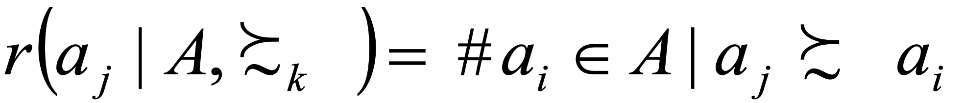
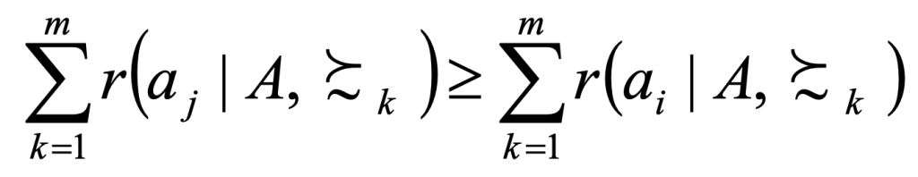
To determine the consensus ranking, the total Borda mark is calculated according to formula 20. The individual marks are summarised for each option and the best (consensus) option is the one with the highest total Borda mark.
An option aj is preferred to another option aj in the final group ranking only if
| Considering a simple example of three decision makers {A,B,C} and three options {a1, a2, a3} A) Initial individual rankings | |||||
| Best options | .. | Worst option | |||
| Decision maker A | a1 | a2 | a3 | ||
| Decision maker B | a2 | a1 | a3 | ||
| Decision maker C | a2 | a3 | a1 | ||
| B) Individual Borda mark | |||||
| Option a1 | a2 | Option a3 | |||
| Decision maker A | 2 | 1 | 0 | ||
| Decision maker B | 1 | 2 | 0 | ||
| Decision maker C | 0 | 2 | 1 | ||
| C) Total Borda mark | |||||
| Option a1 | a2 | a3 | |||
| Total Borda mark | 3 | 5 | 1 | ||
| D) Final ranking Since the highest Borda mark has been assigned to the option a2 and the second highest to the option a1 , the group ranking is | |||||
3.3 ALTERNATIVE GROUP RANKING
In the mDSS4 a few alternative group decision algorithms have been implemented. Condorcet winner (called after the mathematician and philosopher Marie Jean Antoine Nicolas Caritat, the Marquis de Condorcet) is an option that, when compared individually with each of the alternative options, is preferred by a majority of voters. The Condorcet winner is estimated by a series of imaginary pairwise contests. In each contest, the winning option is the one that the majority of voters rank higher than the alternative (decision makers, stakeholders). When all possible pairs of options have been considered, the option that beats every other option in these contests is declared the Condorcet winner. Due to cyclic collective preferences, there may be no Condorcet winner. In such a case other group decision methods need to be applied.
The second algorithm for group decision making added to mDSS5 resembles the OWA rule. Following this method, a new set of weights is assigned to different rank positions. The weight vectors are assumed to be decreasing with the highest weight being assigned to the top position of the option ranks. Depending on the actual values of the weights, several strategies can be distinguished:
- Plurality voting: (1, 0, 0, …, 0):All rank positions but the first are given weight 0. The winner is the alternative that is placed at the first position in the orders by the greatest number of experts.
- Anti-plurality voting (1, 1, 1, …, 0): All rank positions but the latest are given weight 1. In this method, the experts indirectly point out the alternative judged as the worst one. The winner is the alternative that is placed at the last position in the orders by the least number of experts.
- Z–plurality method (1,1, …., n – z = 1, 0, 0, …, 0): The first n-z rank positions are assigned the weight 1 (n = number of options, z = arbitrary chosen number, n > z). It is easy to show that if z = n – 1, plurality voting is produced, and if z = 1, the corresponding results are equal to the anti-plurality strategy.
To calculate collective preference, the weights are multiplied by the number of times an option was ranked at a certain position.